
Data Visualization - Kaggle 官方课程
来源:Kaggle 官方课程 Data Visualization
2024-09-01@isSeymour
Data Visualization
总览:
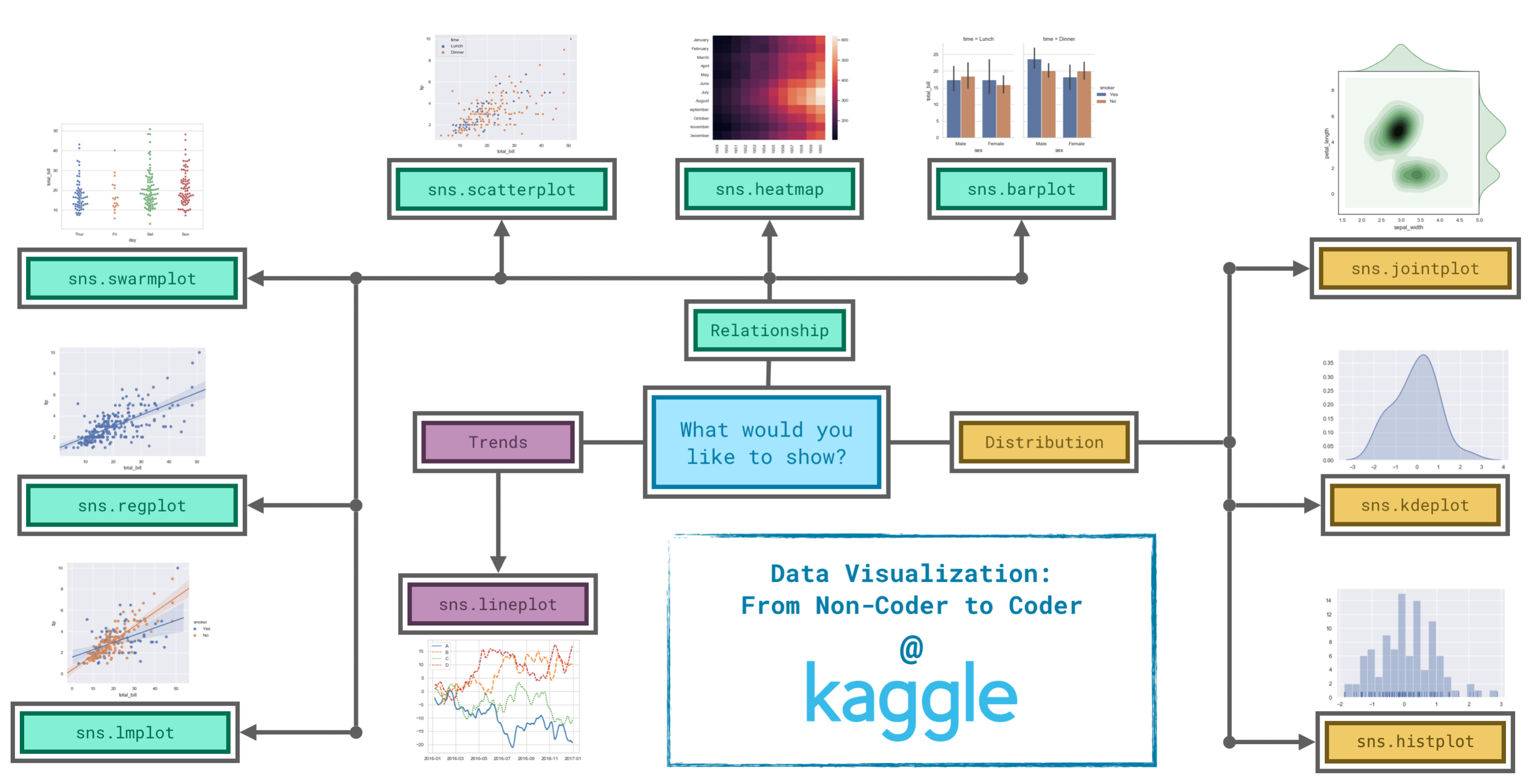
展现内容:
-
Trends 趋势
代码 功能 lineplot 折线图用于展示数据随时间或其他连续变量的变化趋势 -
Relationship 关系
代码 功能 barplot 柱状图用于展示不同类别或分组数据的数量或频率 heatmap 热图用于显示数据的密度或强度,通过颜色的深浅来表示数值的大小 scatterplot 散点图用于展示两个变量之间关系 swarmplot 蜂群图用于显示数据分布的可视化图表,通过将数据点以散点的方式展示在类别上,并避免数据点重叠。它适用于展示单变量或多变量的离散数据分布,特别是当数据量较小或希望看到每个数据点的具体位置时 regplot 回归图用于展示回归分析结果的数据可视化工具。它通常包括一个散点图和一条回归线,帮助直观地展示两个变量之间的关系及其回归模型的拟合效果 lmplot 线性回归图用于展示线性回归分析结果的可视化工具。它通过将散点图和线性回归线结合在一起,帮助直观地理解自变量与因变量之间的线性关系 -
Distribution 分布
代码 功能 jointplot 联合图是一种综合了散点图和边际直方图的数据可视化工具,用于展示两个变量之间的关系及其各自的分布情况。联合图通过将散点图与边际分布图结合,提供了对数据关系和分布的全面视角 kdeplot 核密度估计图用于估计和可视化数据分布的图表。它通过核密度估计方法将数据的概率密度函数平滑化,提供了数据分布的平滑估计 histplot 直方图用于展示数据分布情况的图表。它通过将数据分成多个区间(或称为“桶”)并计算每个区间中的数据点数目,直观地表示了数据的分布情况
0. 导入库
1 | import pandas as pd |
Setup Complete
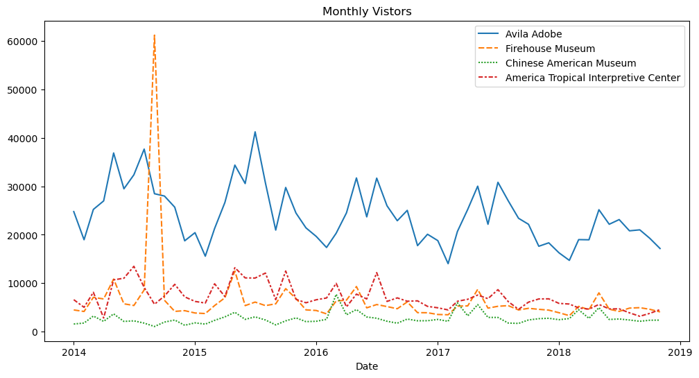
1. Trends 趋势
1 | museum_filepath = "../input/museum_visitors.csv" |
Shape: (59, 4)
| Avila Adobe | Firehouse Museum | Chinese American Museum | America Tropical Interpretive Center | |
|---|---|---|---|---|
| Date | ||||
| 2018-07-01 | 23136 | 4191 | 2620 | 4718 |
| 2018-08-01 | 20815 | 4866 | 2409 | 3891 |
| 2018-09-01 | 21020 | 4956 | 2146 | 3180 |
| 2018-10-01 | 19280 | 4622 | 2364 | 3775 |
| 2018-11-01 | 17163 | 4082 | 2385 | 4562 |
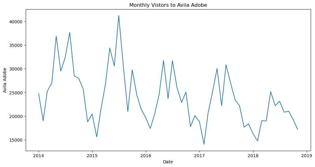
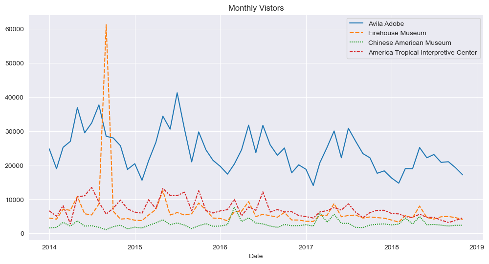
1 | # 折线图 |
Text(0.5, 1.0, 'Monthly Vistors')
1 | # 折线图 |
Text(0.5, 0, 'Date')
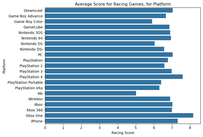
2. Relationship 关系
1 | ign_filepath = "../input/ign_scores.csv" |
Shape: (21, 12)
| Action | Action, Adventure | Adventure | Fighting | Platformer | Puzzle | RPG | Racing | Shooter | Simulation | Sports | Strategy | |
|---|---|---|---|---|---|---|---|---|---|---|---|---|
| Platform | ||||||||||||
| Dreamcast | 6.882857 | 7.511111 | 6.281818 | 8.200000 | 8.340000 | 8.088889 | 7.700000 | 7.042500 | 7.616667 | 7.628571 | 7.272222 | 6.433333 |
| Game Boy Advance | 6.373077 | 7.507692 | 6.057143 | 6.226316 | 6.970588 | 6.532143 | 7.542857 | 6.657143 | 6.444444 | 6.928571 | 6.694444 | 7.175000 |
| Game Boy Color | 6.272727 | 8.166667 | 5.307692 | 4.500000 | 6.352941 | 6.583333 | 7.285714 | 5.897436 | 4.500000 | 5.900000 | 5.790698 | 7.400000 |
| GameCube | 6.532584 | 7.608333 | 6.753846 | 7.422222 | 6.665714 | 6.133333 | 7.890909 | 6.852632 | 6.981818 | 8.028571 | 7.481319 | 7.116667 |
| Nintendo 3DS | 6.670833 | 7.481818 | 7.414286 | 6.614286 | 7.503448 | 8.000000 | 7.719231 | 6.900000 | 7.033333 | 7.700000 | 6.388889 | 7.900000 |
| Nintendo 64 | 6.649057 | 8.250000 | 7.000000 | 5.681250 | 6.889655 | 7.461538 | 6.050000 | 6.939623 | 8.042857 | 5.675000 | 6.967857 | 6.900000 |
| Nintendo DS | 5.903608 | 7.240000 | 6.259804 | 6.320000 | 6.840000 | 6.604615 | 7.222619 | 6.038636 | 6.965217 | 5.874359 | 5.936667 | 6.644737 |
| Nintendo DSi | 6.827027 | 8.500000 | 6.090909 | 7.500000 | 7.250000 | 6.810526 | 7.166667 | 6.563636 | 6.500000 | 5.195652 | 5.644444 | 6.566667 |
| PC | 6.805791 | 7.334746 | 7.136798 | 7.166667 | 7.410938 | 6.924706 | 7.759930 | 7.032418 | 7.084878 | 7.104889 | 6.902424 | 7.310207 |
| PlayStation | 6.016406 | 7.933333 | 6.313725 | 6.553731 | 6.579070 | 6.757895 | 7.910000 | 6.773387 | 6.424000 | 6.918182 | 6.751220 | 6.496875 |
| PlayStation 2 | 6.467361 | 7.250000 | 6.315152 | 7.306349 | 7.068421 | 6.354545 | 7.473077 | 6.585065 | 6.641667 | 7.152632 | 7.197826 | 7.238889 |
| PlayStation 3 | 6.853819 | 7.306154 | 6.820988 | 7.710938 | 7.735714 | 7.350000 | 7.436111 | 6.978571 | 7.219553 | 7.142857 | 7.485816 | 7.355172 |
| PlayStation 4 | 7.550000 | 7.835294 | 7.388571 | 7.280000 | 8.390909 | 7.400000 | 7.944000 | 7.590000 | 7.804444 | 9.250000 | 7.430000 | 6.566667 |
| PlayStation Portable | 6.467797 | 7.000000 | 6.938095 | 6.822222 | 7.194737 | 6.726667 | 6.817778 | 6.401961 | 7.071053 | 6.761538 | 6.956790 | 6.550000 |
| PlayStation Vita | 7.173077 | 6.133333 | 8.057143 | 7.527273 | 8.568750 | 8.250000 | 7.337500 | 6.300000 | 7.660000 | 5.725000 | 7.130000 | 8.900000 |
| Wii | 6.262718 | 7.294643 | 6.234043 | 6.733333 | 7.054255 | 6.426984 | 7.410345 | 5.011667 | 6.479798 | 6.327027 | 5.966901 | 6.975000 |
| Wireless | 7.041699 | 7.312500 | 6.972414 | 6.740000 | 7.509091 | 7.360550 | 8.260000 | 6.898305 | 6.906780 | 7.802857 | 7.417699 | 7.542857 |
| Xbox | 6.819512 | 7.479032 | 6.821429 | 7.029630 | 7.303448 | 5.125000 | 8.277778 | 7.021591 | 7.485417 | 7.155556 | 7.884397 | 7.313333 |
| Xbox 360 | 6.719048 | 7.137838 | 6.857353 | 7.552239 | 7.559574 | 7.141026 | 7.650000 | 6.996154 | 7.338153 | 7.325000 | 7.317857 | 7.112245 |
| Xbox One | 7.702857 | 7.566667 | 7.254545 | 7.171429 | 6.733333 | 8.100000 | 8.291667 | 8.163636 | 8.020000 | 7.733333 | 7.331818 | 8.500000 |
| iPhone | 6.865445 | 7.764286 | 7.745833 | 6.087500 | 7.471930 | 7.810784 | 7.185185 | 7.315789 | 6.995588 | 7.328571 | 7.152174 | 7.534921 |
1 | # 柱状图 |
Text(0.5, 0, 'Racing Score')
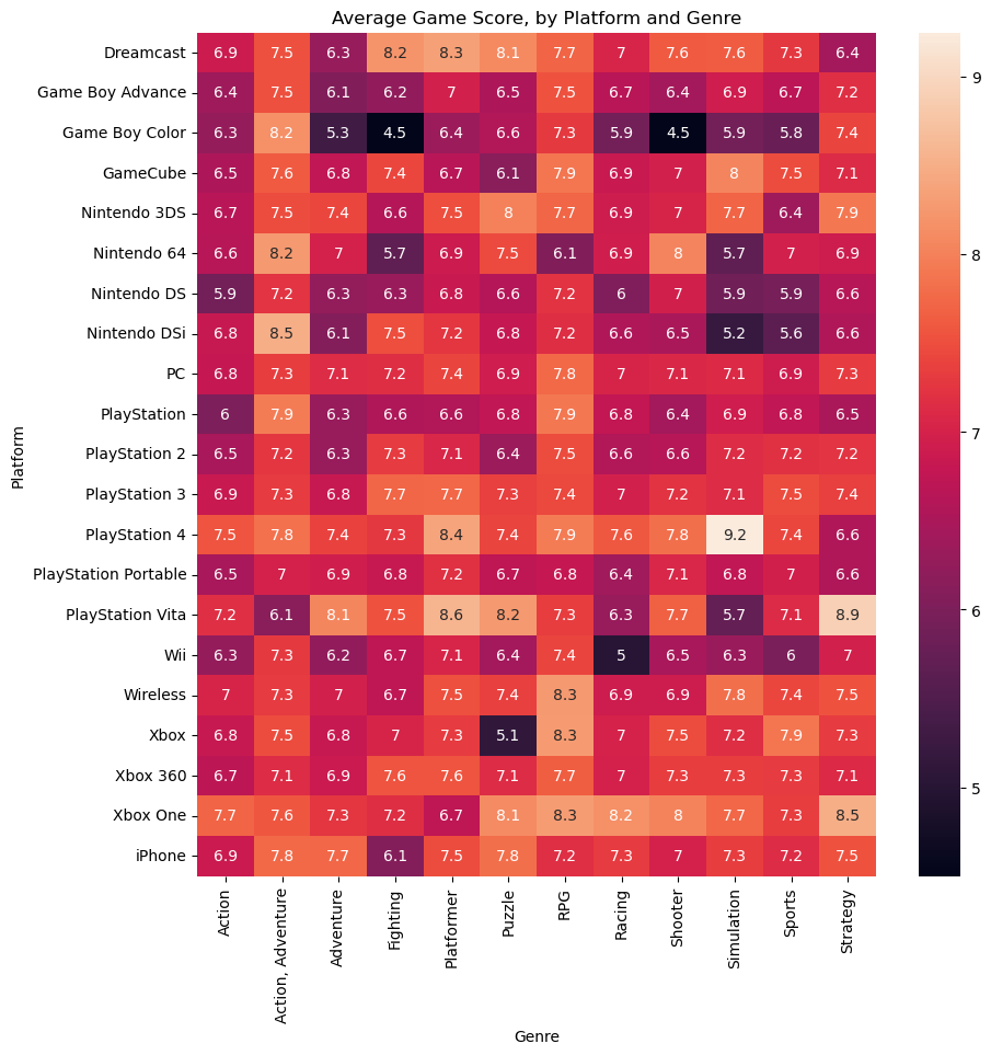
1 | # 热图 |
Text(0.5, 80.7222222222222, 'Genre')
1 | candy_filepath = "../input/candy.csv" |
Shape: (83, 13)
| competitorname | chocolate | fruity | caramel | peanutyalmondy | nougat | crispedricewafer | hard | bar | pluribus | sugarpercent | pricepercent | winpercent | |
|---|---|---|---|---|---|---|---|---|---|---|---|---|---|
| id | |||||||||||||
| 0 | 100 Grand | Yes | No | Yes | No | No | Yes | No | Yes | No | 0.732 | 0.860 | 66.971725 |
| 1 | 3 Musketeers | Yes | No | No | No | Yes | No | No | Yes | No | 0.604 | 0.511 | 67.602936 |
| 2 | Air Heads | No | Yes | No | No | No | No | No | No | No | 0.906 | 0.511 | 52.341465 |
| 3 | Almond Joy | Yes | No | No | Yes | No | No | No | Yes | No | 0.465 | 0.767 | 50.347546 |
| 4 | Baby Ruth | Yes | No | Yes | Yes | Yes | No | No | Yes | No | 0.604 | 0.767 | 56.914547 |
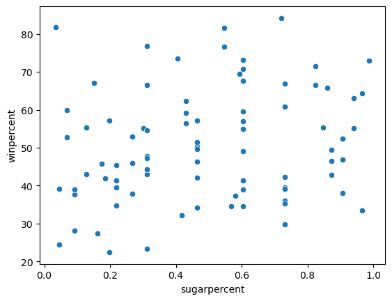
1 | # 散点图 |
<Axes: xlabel='sugarpercent', ylabel='winpercent'>
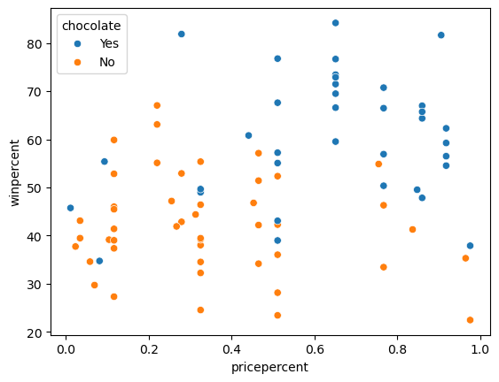
1 | # 散点图 |
<Axes: xlabel='pricepercent', ylabel='winpercent'>
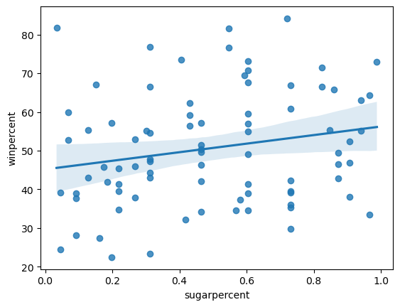
1 | # 回归图 |
<Axes: xlabel='sugarpercent', ylabel='winpercent'>
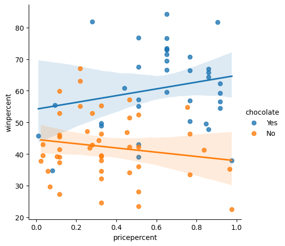
1 | # 线性回归图 |
<seaborn.axisgrid.FacetGrid at 0x163884c10>
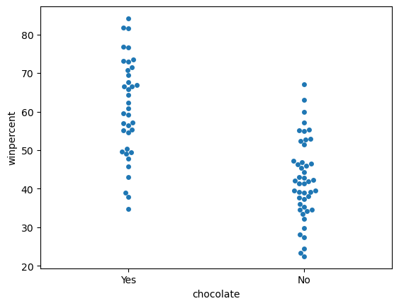
1 | # 蜂群图 |
<Axes: xlabel='chocolate', ylabel='winpercent'>
3. Distributions 分布
1 | cancer_filepath = '../input/cancer.csv' |
Shape: (569, 31)
| Diagnosis | Radius (mean) | Texture (mean) | Perimeter (mean) | Area (mean) | Smoothness (mean) | Compactness (mean) | Concavity (mean) | Concave points (mean) | Symmetry (mean) | ... | Radius (worst) | Texture (worst) | Perimeter (worst) | Area (worst) | Smoothness (worst) | Compactness (worst) | Concavity (worst) | Concave points (worst) | Symmetry (worst) | Fractal dimension (worst) | |
|---|---|---|---|---|---|---|---|---|---|---|---|---|---|---|---|---|---|---|---|---|---|
| Id | |||||||||||||||||||||
| 8510426 | B | 13.540 | 14.36 | 87.46 | 566.3 | 0.09779 | 0.08129 | 0.06664 | 0.047810 | 0.1885 | ... | 15.110 | 19.26 | 99.70 | 711.2 | 0.14400 | 0.17730 | 0.23900 | 0.12880 | 0.2977 | 0.07259 |
| 8510653 | B | 13.080 | 15.71 | 85.63 | 520.0 | 0.10750 | 0.12700 | 0.04568 | 0.031100 | 0.1967 | ... | 14.500 | 20.49 | 96.09 | 630.5 | 0.13120 | 0.27760 | 0.18900 | 0.07283 | 0.3184 | 0.08183 |
| 8510824 | B | 9.504 | 12.44 | 60.34 | 273.9 | 0.10240 | 0.06492 | 0.02956 | 0.020760 | 0.1815 | ... | 10.230 | 15.66 | 65.13 | 314.9 | 0.13240 | 0.11480 | 0.08867 | 0.06227 | 0.2450 | 0.07773 |
| 854941 | B | 13.030 | 18.42 | 82.61 | 523.8 | 0.08983 | 0.03766 | 0.02562 | 0.029230 | 0.1467 | ... | 13.300 | 22.81 | 84.46 | 545.9 | 0.09701 | 0.04619 | 0.04833 | 0.05013 | 0.1987 | 0.06169 |
| 85713702 | B | 8.196 | 16.84 | 51.71 | 201.9 | 0.08600 | 0.05943 | 0.01588 | 0.005917 | 0.1769 | ... | 8.964 | 21.96 | 57.26 | 242.2 | 0.12970 | 0.13570 | 0.06880 | 0.02564 | 0.3105 | 0.07409 |
5 rows × 31 columns
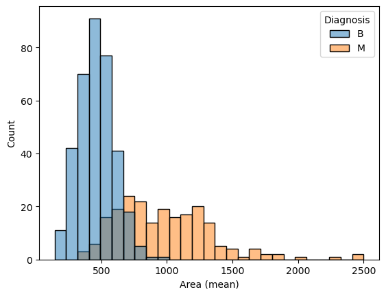
1 | # Histogram 直方图 |
<Axes: xlabel='Area (mean)', ylabel='Count'>
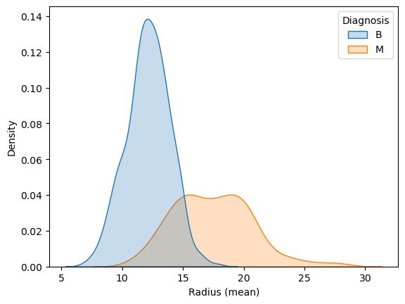
1 | # KDE 核密度估计图 |
<Axes: xlabel='Radius (mean)', ylabel='Density'>
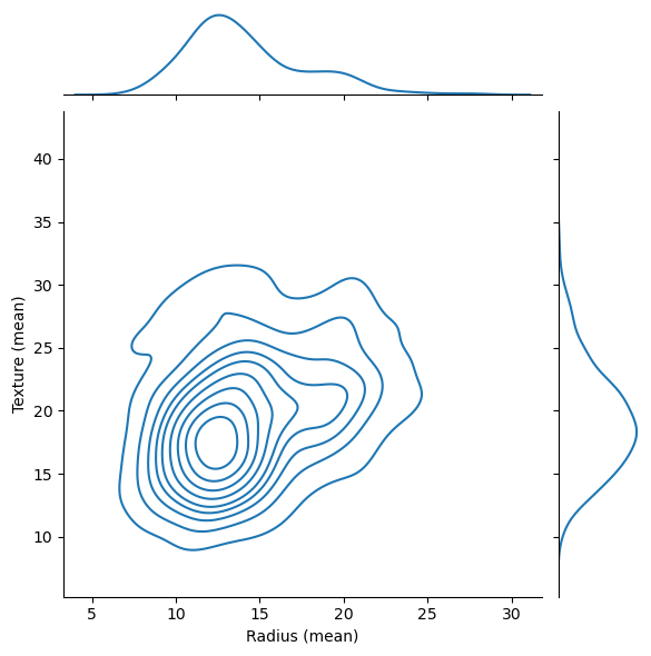
1 | # joint Plot 联合图 |
<seaborn.axisgrid.JointGrid at 0x163ab5190>
Custom Styles 自定义样式
1 | # (1)"darkgrid", (2)"whitegrid", (3)"dark", (4)"white", and (5)"ticks" |
Text(0.5, 1.0, 'Monthly Vistors')
本博客所有文章除特别声明外,均采用 CC BY-NC-SA 4.0 许可协议。转载请注明来自 isSeymour!
 微信支付
微信支付 支付宝
支付宝
相关推荐


评论