来源:Kaggle 官方课程 Intro to Deep Learning
Intro to Deep Learning
Exercise: Binary Classification
1.导入数据
1
2
3
4
5
6
7
8
9
10
11
12
import pandas as pdimport matplotlib.pyplot as pltfrom sklearn.model_selection import train_test_splitfrom sklearn.preprocessing import StandardScaler, OneHotEncoderfrom sklearn.impute import SimpleImputerfrom sklearn.pipeline import make_pipelinefrom sklearn.compose import make_column_transformerhotel = pd.read_csv('../input/hotel.csv' ) print ("Shape: " , hotel.shape)hotel.head()
Shape: (119390, 32)
hotel
is_canceled
lead_time
arrival_date_year
arrival_date_month
arrival_date_week_number
arrival_date_day_of_month
stays_in_weekend_nights
stays_in_week_nights
adults
...
deposit_type
agent
company
days_in_waiting_list
customer_type
adr
required_car_parking_spaces
total_of_special_requests
reservation_status
reservation_status_date
0
Resort Hotel
0
342
2015
July
27
1
0
0
2
...
No Deposit
NaN
NaN
0
Transient
0.0
0
0
Check-Out
2015-07-01
1
Resort Hotel
0
737
2015
July
27
1
0
0
2
...
No Deposit
NaN
NaN
0
Transient
0.0
0
0
Check-Out
2015-07-01
2
Resort Hotel
0
7
2015
July
27
1
0
1
1
...
No Deposit
NaN
NaN
0
Transient
75.0
0
0
Check-Out
2015-07-02
3
Resort Hotel
0
13
2015
July
27
1
0
1
1
...
No Deposit
304.0
NaN
0
Transient
75.0
0
0
Check-Out
2015-07-02
4
Resort Hotel
0
14
2015
July
27
1
0
2
2
...
No Deposit
240.0
NaN
0
Transient
98.0
0
1
Check-Out
2015-07-03
5 rows × 32 columns
2. 数据清洗
1
2
3
4
5
6
7
8
9
10
11
12
13
14
15
16
17
18
19
20
21
22
23
24
25
26
27
28
29
30
31
32
33
34
35
36
37
38
39
40
41
42
43
44
45
46
47
48
49
50
51
52
53
54
55
56
57
58
59
60
X = hotel.copy() y = X.pop('is_canceled' ) X['arrival_date_month' ] = \ X['arrival_date_month' ].map ( {'January' :1 , 'February' : 2 , 'March' :3 , 'April' :4 , 'May' :5 , 'June' :6 , 'July' :7 , 'August' :8 , 'September' :9 , 'October' :10 , 'November' :11 , 'December' :12 } ) features_num = [ "lead_time" , "arrival_date_week_number" , "arrival_date_day_of_month" , "stays_in_weekend_nights" , "stays_in_week_nights" , "adults" , "children" , "babies" , "is_repeated_guest" , "previous_cancellations" , "previous_bookings_not_canceled" , "required_car_parking_spaces" , "total_of_special_requests" , "adr" , ] features_cat = [ "hotel" , "arrival_date_month" , "meal" , "market_segment" , "distribution_channel" , "reserved_room_type" , "deposit_type" , "customer_type" , ] transformer_num = make_pipeline( SimpleImputer(strategy="constant" ), StandardScaler(), ) transformer_cat = make_pipeline( SimpleImputer(strategy="constant" , fill_value="NA" ), OneHotEncoder(handle_unknown='ignore' ), ) preprocessor = make_column_transformer( (transformer_num, features_num), (transformer_cat, features_cat), ) X_train, X_valid, y_train, y_valid = \ train_test_split(X, y, stratify=y, train_size=0.75 ) X_train = preprocessor.fit_transform(X_train) X_valid = preprocessor.transform(X_valid) input_shape = [X_train.shape[1 ]]
3. 定义模型、损失函数、优化器
1
2
3
4
5
6
7
8
9
10
11
12
13
14
15
16
17
18
19
20
21
22
23
24
25
26
27
28
29
30
31
32
33
34
35
36
37
38
39
40
41
42
43
44
45
46
47
48
49
50
51
52
53
54
55
56
57
58
import torchimport torch.nn as nnimport torch.optim as optimfrom torch.utils.data import DataLoader, TensorDatasetclass MyModel (nn.Module): def __init__ (self, input_shape ): super (MyModel, self).__init__() self.model = nn.Sequential( nn.BatchNorm1d(input_shape), nn.Linear(input_shape, 256 ), nn.ReLU(), nn.BatchNorm1d(256 ), nn.Dropout(0.3 ), nn.Linear(256 , 256 ), nn.ReLU(), nn.BatchNorm1d(256 ), nn.Dropout(0.3 ), nn.Linear(256 , 1 ), nn.Sigmoid() ) def forward (self, x ): return self.model(x) input_shape = X_train.shape[1 ] model = MyModel(input_shape) criterion = nn.BCELoss() optimizer = optim.Adam(model.parameters(), lr=0.001 ) if isinstance (X_train, pd.DataFrame) or isinstance (X_train, pd.Series): X_train = X_train.values if isinstance (y_train, pd.DataFrame) or isinstance (y_train, pd.Series): y_train = y_train.values if isinstance (X_valid, pd.DataFrame) or isinstance (X_valid, pd.Series): X_valid = X_valid.values if isinstance (y_valid, pd.DataFrame) or isinstance (y_valid, pd.Series): y_valid = y_valid.values X_train_tensor = torch.tensor(X_train, dtype=torch.float32) y_train_tensor = torch.tensor(y_train, dtype=torch.float32) X_valid_tensor = torch.tensor(X_valid, dtype=torch.float32) y_valid_tensor = torch.tensor(y_valid, dtype=torch.float32) train_dataset = TensorDataset(X_train_tensor, y_train_tensor) valid_dataset = TensorDataset(X_valid_tensor, y_valid_tensor) train_loader = DataLoader(train_dataset, batch_size=512 , shuffle=True ) valid_loader = DataLoader(valid_dataset, batch_size=512 , shuffle=False )
4. 训练模型
1 2 3 4 5 6 7 8 9 10 11 12 13 14 15 16 17 18 19 20 21 22 23 24 25 26 27 28 29 30 31 32 33 34 35 36 37 38 39 40 41 42 43 44 45 46 47 48 epochs = 20 train_loss_history = [] valid_loss_history = [] train_acc_history = [] valid_acc_history = [] for epoch in range (epochs): model.train() train_loss = 0 correct = 0 total = 0 for inputs, targets in train_loader: optimizer.zero_grad() outputs = model(inputs).squeeze() loss = criterion(outputs, targets) loss.backward() optimizer.step() train_loss += loss.item() * inputs.size(0 ) predicted = (outputs > 0.5 ).float () correct += (predicted == targets).sum ().item() total += targets.size(0 ) train_loss /= total train_acc = correct / total train_loss_history.append(train_loss) train_acc_history.append(train_acc) model.eval () valid_loss = 0 correct = 0 total = 0 with torch.no_grad(): for inputs, targets in valid_loader: outputs = model(inputs).squeeze() loss = criterion(outputs, targets) valid_loss += loss.item() * inputs.size(0 ) predicted = (outputs > 0.5 ).float () correct += (predicted == targets).sum ().item() total += targets.size(0 ) valid_loss /= total valid_acc = correct / total valid_loss_history.append(valid_loss) valid_acc_history.append(valid_acc) print (f"Epoch {epoch+1 } /{epochs} - Loss: {train_loss:.4 f} , Accuracy: {train_acc:.4 f} , Val Loss: {valid_loss:.4 f} , Val Accuracy: {valid_acc:.4 f} " )
Epoch 1/20 - Loss: 0.4443, Accuracy: 0.7889, Val Loss: 0.4133, Val Accuracy: 0.8053
Epoch 2/20 - Loss: 0.4100, Accuracy: 0.8080, Val Loss: 0.3998, Val Accuracy: 0.8106
Epoch 3/20 - Loss: 0.4000, Accuracy: 0.8129, Val Loss: 0.3966, Val Accuracy: 0.8168
Epoch 4/20 - Loss: 0.3934, Accuracy: 0.8168, Val Loss: 0.3875, Val Accuracy: 0.8167
Epoch 5/20 - Loss: 0.3886, Accuracy: 0.8197, Val Loss: 0.3830, Val Accuracy: 0.8240
Epoch 6/20 - Loss: 0.3844, Accuracy: 0.8210, Val Loss: 0.3817, Val Accuracy: 0.8239
Epoch 7/20 - Loss: 0.3794, Accuracy: 0.8249, Val Loss: 0.3814, Val Accuracy: 0.8252
Epoch 8/20 - Loss: 0.3761, Accuracy: 0.8262, Val Loss: 0.3743, Val Accuracy: 0.8283
Epoch 9/20 - Loss: 0.3738, Accuracy: 0.8278, Val Loss: 0.3762, Val Accuracy: 0.8282
Epoch 10/20 - Loss: 0.3713, Accuracy: 0.8290, Val Loss: 0.3709, Val Accuracy: 0.8290
Epoch 11/20 - Loss: 0.3678, Accuracy: 0.8299, Val Loss: 0.3697, Val Accuracy: 0.8312
Epoch 12/20 - Loss: 0.3655, Accuracy: 0.8320, Val Loss: 0.3705, Val Accuracy: 0.8309
Epoch 13/20 - Loss: 0.3639, Accuracy: 0.8321, Val Loss: 0.3681, Val Accuracy: 0.8310
Epoch 14/20 - Loss: 0.3629, Accuracy: 0.8330, Val Loss: 0.3676, Val Accuracy: 0.8317
Epoch 15/20 - Loss: 0.3596, Accuracy: 0.8337, Val Loss: 0.3653, Val Accuracy: 0.8320
Epoch 16/20 - Loss: 0.3581, Accuracy: 0.8353, Val Loss: 0.3651, Val Accuracy: 0.8319
Epoch 17/20 - Loss: 0.3560, Accuracy: 0.8354, Val Loss: 0.3611, Val Accuracy: 0.8338
Epoch 18/20 - Loss: 0.3559, Accuracy: 0.8362, Val Loss: 0.3664, Val Accuracy: 0.8335
Epoch 19/20 - Loss: 0.3541, Accuracy: 0.8371, Val Loss: 0.3653, Val Accuracy: 0.8333
Epoch 20/20 - Loss: 0.3513, Accuracy: 0.8384, Val Loss: 0.3596, Val Accuracy: 0.8349
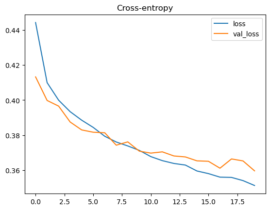
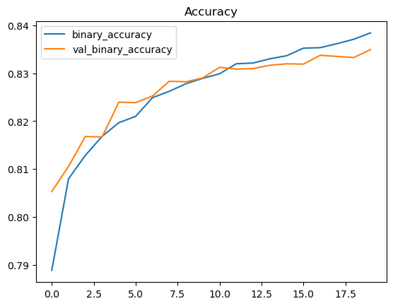
5. 训练可视化
1 2 3 4 5 6 7 8 9 10 11 12 13 history_df = pd.DataFrame({ 'loss' : train_loss_history, 'val_loss' : valid_loss_history, 'binary_accuracy' : train_acc_history, 'val_binary_accuracy' : valid_acc_history, }) history_df[['loss' , 'val_loss' ]].plot(title="Cross-entropy" ) plt.show() history_df[['binary_accuracy' , 'val_binary_accuracy' ]].plot(title="Accuracy" ) plt.show()

 微信支付
微信支付 支付宝
支付宝