CS224W - Colab 1
CS224W - Colab 1
In this Colab, we will write a full pipeline for learning node embeddings.
We will go through the following 3 steps.
To start, we will load a classic graph in network science, the Karate Club Network. We will explore multiple graph statistics for that graph.
We will then work together to transform the graph structure into a PyTorch tensor, so that we can perform machine learning over the graph.
Finally, we will finish the first learning algorithm on graphs: a node embedding model. For simplicity, our model here is simpler than DeepWalk / node2vec algorithms taught in the lecture. But it’s still rewarding and challenging, as we will write it from scratch via PyTorch.
Now let’s get started! This Colab should take 1-2 hours to complete.
Note: Make sure to restart and run all before submission, so that the intermediate variables / packages will carry over to the next cell
1 Graph Basics
To start, we will load a classic graph in network science, the Karate Club Network. We will explore multiple graph statistics for that graph.
Setup
We will heavily use NetworkX in this Colab.
1 | import networkx as nx |
Zachary’s karate club network
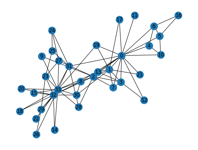
The Karate Club Network is a graph which describes a social network of 34 members of a karate club and documents links between members who interacted outside the club.
1 | G = nx.karate_club_graph() |
networkx.classes.graph.Graph
1 | # Visualize the graph |
Question 1: What is the average degree of the karate club network? (5 Points)
1 | def average_degree(num_edges, num_nodes): |
Average degree of karate club network is 5
Question 2: What is the average clustering coefficient of the karate club network? (5 Points)
1 | def average_clustering_coefficient(G): |
Average clustering coefficient of karate club network is 0.57
Question 3: What is the PageRank value for node 0 (node with id 0) after one PageRank iteration? (5 Points)
Page Rank measures importance of nodes in a graph using the link structure of the web. A “vote” from an important page is worth more. Specifically, if a page with importance has out-links, then each link gets votes. Thus, the importance of a Page , represented as is the sum of the votes on its in links.
r_j = \sum_{i \rightarrow j} \frac{r_i}{d_i}$$, where $d_i$ is the out degree of node $i$. The PageRank algorithm (used by Google) outputs a probability distribution which represent the likelihood of a random surfer clicking on links will arrive at any particular page. At each time step, the random surfer has two options - With prob. $\beta$, follow a link at random - With prob. $1- \beta$, jump to a random page Thus, the importance of a particular page is calculated with the following PageRank equation: $$r_j = \sum_{i \rightarrow j} \beta \frac{r_i}{d_i} + (1 - \beta) \frac{1}{N}
Please complete the code block by implementing the above PageRank equation for node 0.
Note - You can refer to more information from the slides here - http://snap.stanford.edu/class/cs224w-2020/slides/04-pagerank.pdf
1 | def one_iter_pagerank(G, beta, r0, node_id): |
The PageRank value for node 0 after one iteration is 0.13
Question 4: What is the (raw) closeness centrality for the karate club network node 5? (5 Points)
The equation for closeness centrality is
1 | def closeness_centrality(G, node=5): |
The node 5 has closeness centrality 0.38
2 Graph to Tensor
We will then work together to transform the graph into a PyTorch tensor, so that we can perform machine learning over the graph.
Setup
Check if PyTorch is properly installed
1 | import torch |
2.4.1
PyTorch tensor basics
We can generate PyTorch tensor with all zeros, ones or random values.
1 | # Generate 3 x 4 tensor with all ones |
tensor([[1., 1., 1., 1.],
        [1., 1., 1., 1.],
        [1., 1., 1., 1.]])
tensor([[0., 0., 0., 0.],
        [0., 0., 0., 0.],
        [0., 0., 0., 0.]])
tensor([[0.5627, 0.2231, 0.4255, 0.7039],
        [0.0281, 0.1933, 0.5920, 0.9510],
        [0.0953, 0.9217, 0.0193, 0.3396]])
torch.Size([3, 4])
PyTorch tensor contains elements for a single data type, the dtype.
1 | # Create a 3 x 4 tensor with all 32-bit floating point zeros |
torch.float32
torch.int64
Question 5: Get the edge list of the karate club network and transform it into torch.LongTensor. What is the torch.sum value of pos_edge_index tensor? (10 Points)
1 | def graph_to_edge_list(G): |
The pos_edge_index tensor has shape torch.Size([2, 78])
The pos_edge_index tensor has sum value 2535
Question 6: Please implement following function that samples negative edges. Then answer which edges (edge_1 to edge_5) are the negative edges in the karate club network? (10 Points)
“Negative” edges refer to the edges/links that do not exist in the graph. The term “negative” is borrowed from “negative sampling” in link prediction. It has nothing to do with the edge weights.
For example, given an edge (src, dst), you should check that neither (src, dst) nor (dst, src) are edges in the Graph. If these hold true, then it is a negative edge.
1 | import random |
The neg_edge_index tensor has shape torch.Size([2, 78])
Edge 1 can be a negative edge: False
Edge 2 can be a negative edge: True
Edge 3 can be a negative edge: False
Edge 4 can be a negative edge: False
Edge 5 can be a negative edge: True
3 Node Emebedding Learning
Finally, we will finish the first learning algorithm on graphs: a node embedding model.
Setup
1 | import torch |
2.4.1
To write our own node embedding learning methods, we’ll heavily use the nn.Embedding module in PyTorch. Let’s see how to use nn.Embedding:
1 | # Initialize an embedding layer |
Sample embedding layer: Embedding(4, 8)
We can select items from the embedding matrix, by using Tensor indices
1 | # Select an embedding in emb_sample |
tensor([[ 0.0643, -0.6521,  0.1235,  0.0435,  0.7306, -0.9286, -0.2463,  0.4538]],
       grad_fn=<EmbeddingBackward0>)
tensor([[ 0.0643, -0.6521,  0.1235,  0.0435,  0.7306, -0.9286, -0.2463,  0.4538],
        [ 0.0295,  3.1822,  2.7626,  0.3644,  0.8467, -0.4309, -1.1269,  0.5526]],
       grad_fn=<EmbeddingBackward0>)
torch.Size([4, 8])
tensor([[1., 1., 1., 1., 1., 1., 1., 1.],
        [1., 1., 1., 1., 1., 1., 1., 1.]], grad_fn=<EmbeddingBackward0>)
Now, it’s your time to create node embedding matrix for the graph we have!
- We want to have 16 dimensional vector for each node in the karate club network.
- We want to initalize the matrix under uniform distribution, in the range of . We suggest you using
torch.rand.
1 | # Please do not change / reset the random seed |
Embedding: Embedding(34, 16)
tensor([[-0.5773,  0.4670, -0.7134,  0.9294, -0.4133,  0.5903,  0.0341, -0.4398,
          0.6678, -0.7630, -0.5291,  0.1199,  0.7933, -0.4285, -0.6089, -0.6384],
        [ 0.4972,  0.3093, -0.2314,  0.9640,  0.2024, -0.2580, -0.0142,  0.9830,
          0.6717, -0.0741,  0.9804,  0.4391, -0.5324, -0.9101,  0.5811,  0.9378]],
       grad_fn=<EmbeddingBackward0>)
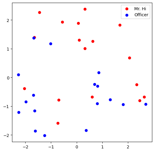
Visualize the initial node embeddings
One good way to understand an embedding matrix, is to visualize it in a 2D space.
Here, we have implemented an embedding visualization function for you.
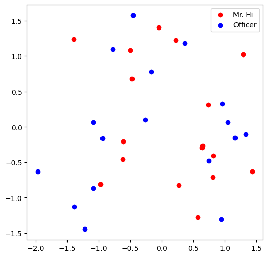
We first do PCA to reduce the dimensionality of embeddings to a 2D space.
Then we visualize each point, colored by the community it belongs to.
1 | def visualize_emb(emb): |
Question 7: Training the embedding! What is the best performance you can get? (20 Points)
We want to optimize our embeddings for the task of classifying edges as positive or negative. Given an edge and the embeddings for each node, the dot product of the embeddings, followed by a sigmoid, should give us the likelihood of that edge being either positive (output of sigmoid > 0.5) or negative (output of sigmoid < 0.5).
Note that we’re using the functions you wrote in the previous questions, as well as the variables initialized in previous cells. If you’re running into issues, make sure your answers to questions 1-6 are correct.
1 | from torch.optim import SGD |
torch.Size([2, 78])
torch.Size([2, 156])
Epoch 0: Loss = 0.9025148153305054, Accuracy = 0.5
Epoch 50: Loss = 0.3298068046569824, Accuracy = 0.9167
Epoch 100: Loss = 0.1502346247434616, Accuracy = 1.0
Epoch 150: Loss = 0.08421747386455536, Accuracy = 1.0
Epoch 200: Loss = 0.05426323041319847, Accuracy = 1.0
Epoch 250: Loss = 0.03854725509881973, Accuracy = 1.0
Epoch 300: Loss = 0.029253864660859108, Accuracy = 1.0
Epoch 350: Loss = 0.02324979566037655, Accuracy = 1.0
Epoch 400: Loss = 0.019109662622213364, Accuracy = 1.0
Epoch 450: Loss = 0.016110926866531372, Accuracy = 1.0


Embedding(34, 16)
Visualize the final node embeddings
Visualize your final embedding here!
You can visually compare the figure with the previous embedding figure.
After training, you should oberserve that the two classes are more evidently separated.
This is a great sanitity check for your implementation as well.
1 | # Visualize the final learned embedding |
Submission
When you submit your assignment, you will have to download this file as an .ipynb file. Please name this file CS224W_Colab_1.ipynb. Make sure that the files are name correctly, otherwise the autograder will not be able to find your submission files.


