参考
精排(二)特征交叉
前面我们讲了Wide & Deep模型,它把记忆能力和泛化能力结合起来。不过Wide部分有个问题:需要人工设计交叉特征,比如“用户年龄×商品类别”这样的组合。这种手工设计的方式不仅费时费力,还很难覆盖所有有用的特征组合。
既然手工设计这么麻烦,那能不能让模型自己学会做特征交叉呢?这就是本节要讨论的核心问题。我们会按照两条技术路线来看:先从简单的二阶交叉开始,然后到更复杂的高阶交叉,最后看看怎么让交叉变得更个性化和自适应。
1、二阶特征交叉
针对 Wide & Deep 模型中人工特征工程的局限性,特征交叉自动化成为了一个迫切需要解决的问题。在这一探索过程中,首先要攻克的是:如何自动、高效地捕捉所有成对(二阶)特征的交互,并将其与深度学习模型结合。 这里的挑战不仅在于"自动",更在于面对推荐场景下海量、高维、稀疏的数据时如何实现"高效"。直接暴力计算所有特征对的组合是不可行的,我们需要一种更巧妙的机制来参数化这些交互。同时,在解决了二阶交互的自动化表达后,如何将这些捕获到的低阶、显式交互信息,与能够学习高阶、隐式关系的深度神经网络(DNN)进行有效融合,也成为这一阶段模型探索的重点。
1.1 FM: 隐向量内积与参数共享
原理
我们在召回章节 已经初步了解了FM ,并见证了它如何作为双塔模型的雏形,通过向量匹配实现召回。在精排阶段,FM的价值得到了更核心的体现。它作为解决特征交叉自动化问题的开创性模型,其核心思想——为每个特征学习一个低维隐向量,并用向量内积来参数化所有二阶交叉项的权重 ——不仅有效解决了参数数量过多和数据稀疏性两大难题,也为这一小节后续模型奠定了方法论的基础。
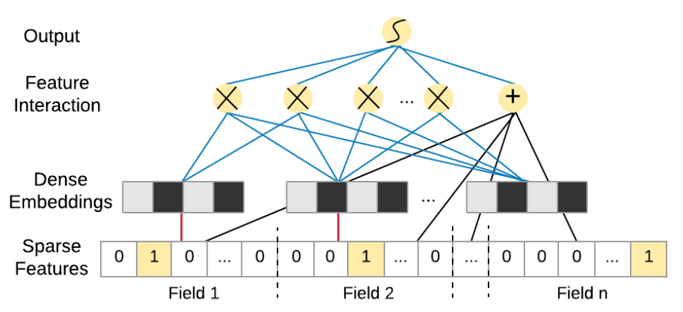
为了捕捉特征间的交互关系,一个直接的想法是在线性模型的基础上增加所有特征的二阶组合项,即多项式模型:
y = w 0 + ∑ i = 1 n w i x i + ∑ i = 1 n − 1 ∑ j = i + 1 n w i j x i x j y = w_0 + \sum_{i=1}^n w_i x_i + \sum_{i=1}^{n-1} \sum_{j=i+1}^n w_{ij} x_i x_j
y = w 0 + i = 1 ∑ n w i x i + i = 1 ∑ n − 1 j = i + 1 ∑ n w ij x i x j
其中,w 0 w_0 w 0 w i w_i w i x i x_i x i w i j w_{ij} w ij x i x_i x i x j x_j x j n n n O ( n 2 ) O(n^2) O ( n 2 ) x i x j x_i x_j x i x j w i j w_{ij} w ij
FM 模型巧妙地解决了这个问题。它将交互权重 w i j w_{ij} w ij w i j = ⟨ v i , v j ⟩ w_{ij}=\langle\mathbf{v}_i,\mathbf{v}_j\rangle w ij = ⟨ v i , v j ⟩
y = w 0 + ∑ i = 1 n w i x i + ∑ i = 1 n − 1 ∑ j = i + 1 n ⟨ v i , v j ⟩ x i x j y = w_0 + \sum_{i=1}^n w_i x_i + \sum_{i=1}^{n-1} \sum_{j=i+1}^n \langle \mathbf{v}_i, \mathbf{v}_j \rangle x_i x_j
y = w 0 + i = 1 ∑ n w i x i + i = 1 ∑ n − 1 j = i + 1 ∑ n ⟨ v i , v j ⟩ x i x j
其中v i , v j \mathbf{v}_i,\mathbf{v}_j v i , v j i i i j j j k k k k k k n n n ⟨ v i , v j ⟩ \langle \mathbf{v}_i,\mathbf{v}_j \rangle ⟨ v i , v j ⟩ ∑ f = 1 k v i , f ⋅ v j , f \sum_{f=1}^k v_{i,f} \cdot v_{j,f} ∑ f = 1 k v i , f ⋅ v j , f
这种参数共享 的设计是 FM 的精髓所在。原本需要学习 O ( n 2 ) O(n^2) O ( n 2 ) w i j w_{ij} w ij k k k v i v_i v i O ( n 2 ) O(n^2) O ( n 2 ) O ( n k ) O(nk) O ( nk ) i i i j j j k k k v i v_i v i v j v_j v j x i x_i x i x j x_j x j O ( k n 2 ) O(kn^2) O ( k n 2 ) O ( k n ) O(kn) O ( kn )
代码
FM的核心在于将 O ( n 2 ) O(n^2) O ( n 2 )
这个实现的巧妙之处在于,无论有多少特征,计算复杂度始终保持线性,使得FM能够处理推荐系统中常见的高维稀疏特征。fm.py 文件:
1
2
3
4
5
6
7
8
9
10
11
12
13
14
15
16
17
18
19
20
21
22
23
24
25
26
27
28
29
30
31
32
33
34
35
36
37
38
39
40
41
42
43
44
45
46
47
48
49
50
51
52
53
54
55
56
57
58
59
60
61
62
63
64
65
66
67
68
69
70
""" 因子分解机(FM)排序模型。 """ import tensorflow as tffrom .utils import ( build_input_layer, build_group_feature_embedding_table_dict, concat_group_embedding, add_tensor_func, get_linear_logits, ) from .layers import FM, PredictLayerdef build_fm_model (feature_columns, model_config ): """ 构建因子分解机(FM)模型 - 用于排序 参数: feature_columns: 特征列配置 model_config: 模型配置字典,包含: - linear_logits: 是否添加线性部分,默认为True """ linear_logits = model_config.get("linear_logits" , True ) input_layer_dict = build_input_layer(feature_columns) group_embedding_feature_dict = build_group_feature_embedding_table_dict( feature_columns, input_layer_dict, prefix="embedding/" ) fm_group_feature_dict = {} for fm_group_name in group_embedding_feature_dict.keys(): concat_fm_feature = concat_group_embedding( group_embedding_feature_dict, fm_group_name, axis=1 , flatten=False ) fm_group_feature_dict[fm_group_name] = concat_fm_feature fm_logit = add_tensor_func( [ FM(name=fm_group_name)(fm_input) for fm_group_name, fm_input in fm_group_feature_dict.items() ] ) if linear_logits: linear_logit = get_linear_logits(input_layer_dict, feature_columns) fm_logit = add_tensor_func([fm_logit, linear_logit], name="fm_linear_logits" ) fm_logit = tf.keras.layers.Flatten()(fm_logit) output = tf.keras.layers.Dense(1 , activation="sigmoid" , name="fm_output" )(fm_logit) output = tf.keras.layers.Flatten()(output) model = tf.keras.models.Model( inputs=list (input_layer_dict.values()), outputs=output ) return model, None , None
1.2 AFM: 注意力加权的交叉特征
原理
FM 对所有特征交叉给予了相同的权重,但实际上不同交叉组合的重要性是不同的。AFM 在此基础上引入注意力机制,为不同的特征交叉分配权重,使模型能关注到更重要的交互。例如,在预测一位用户是否会点击一条体育新闻时,"用户年龄=18-24岁"与"新闻类别=体育"的交叉,其重要性显然要高于"用户年龄=18-24岁"与"新闻发布时间=周三"的交叉。
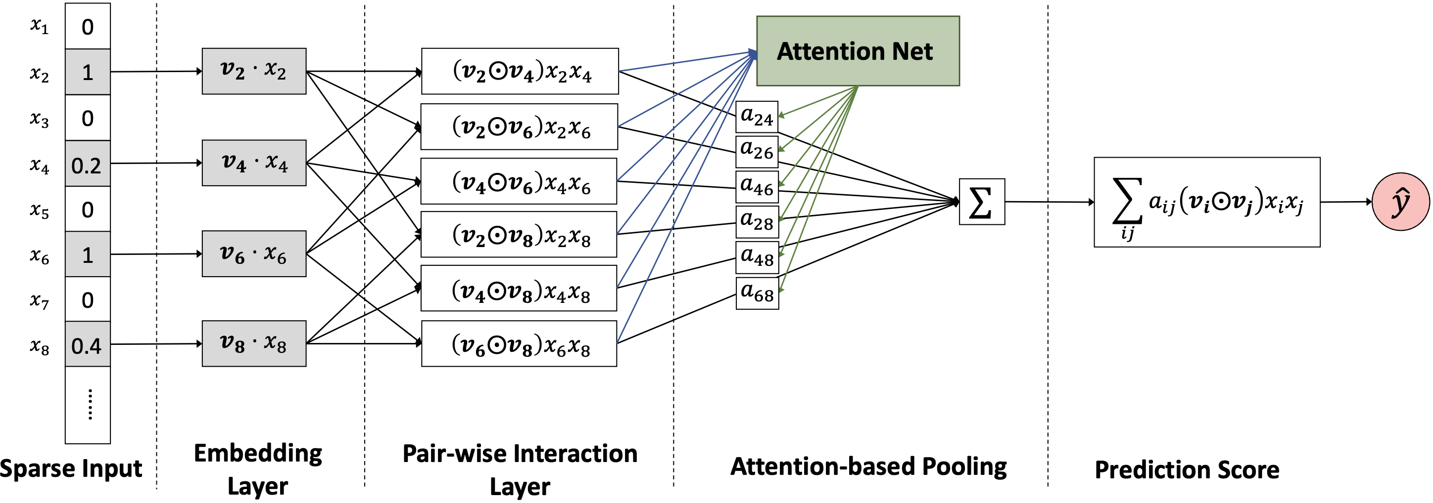
AFM 的模型结构在 FM 的基础上进行了扩展。它首先将所有成对特征的隐向量进行元素积(Hadamard Product, 记为 ⊙ \odot ⊙ ,而不是像 FM 那样直接求内积。这样做保留了交叉特征的向量信息,为后续的注意力计算提供了输入。这个步骤被称为成对交互层(Pair-wise Interaction Layer)。
f P I ( E ) = { ( v i ⊙ v j ) x i x j } ( i , j ) ∈ R x f_{PI}(\mathcal{E}) = \{(v_i \odot v_j) x_i x_j \}_{(i,j) \in \mathcal{R}_x}
f P I ( E ) = {( v i ⊙ v j ) x i x j } ( i , j ) ∈ R x
其中,E \mathcal{E} E R x \mathcal{R}_x R x ( v i ⊙ v j ) (v_i \odot v_j) ( v i ⊙ v j ) a i j a_{ij} a ij
a i j ′ = h T ReLU ( W ( v i ⊙ v j ) x i x j + b ) a i j = exp ( a i j ′ ) ∑ ( i , k ) ∈ R x exp ( a i k ′ ) \begin{aligned}
a_{ij}' &= \textbf{h}^T \text{ReLU}(\textbf{W} (\mathbf{v}_i \odot \mathbf{v}_j) x_i x_j + \textbf{b}) \\
a_{ij} &= \frac{\exp(a_{ij}')}{\sum_{(i,k) \in \mathcal{R}_x} \exp(a_{ik}')}
\end{aligned}
a ij ′ a ij = h T ReLU ( W ( v i ⊙ v j ) x i x j + b ) = ∑ ( i , k ) ∈ R x exp ( a ik ′ ) exp ( a ij ′ )
其中,W \textbf{W} W b \textbf{b} b h \textbf{h} h a i j a_{ij} a ij
f A t t = ∑ ( i , j ) ∈ R x a i j ( v i ⊙ v j ) x i x j f_{Att} = \sum_{(i,j) \in \mathcal{R}_x} a_{ij} (\mathbf{v}_i \odot \mathbf{v}_j) x_i x_j
f A tt = ( i , j ) ∈ R x ∑ a ij ( v i ⊙ v j ) x i x j
最后,AFM 的完整预测公式由一阶线性部分和经过注意力加权的二阶交叉部分组成:
y ^ a f m ( x ) = w 0 + ∑ i = 1 n w i x i + p T f A t t \hat{y}_{afm}(x) = w_0 + \sum_{i=1}^n w_i x_i + \textbf{p}^T f_{Att}
y ^ a f m ( x ) = w 0 + i = 1 ∑ n w i x i + p T f A tt
其中 p \textbf{p} p AFM 不仅提升了模型的表达能力,还通过可视化注意力权重 a i j a_{ij} a ij 赋予了模型更好的可解释性 ,让我们可以洞察哪些特征交叉对预测结果的贡献最大。
代码
AFM的关键在于注意力池化层,它为每个特征交叉对分配不同的权重。
相比FM对所有特征交叉一视同仁,AFM通过注意力机制自动识别重要的交互模式,提升了模型的表达能力和可解释性。afm.py 文件:
1
2
3
4
5
6
7
8
9
10
11
12
13
14
15
16
17
18
19
20
21
22
23
24
25
26
27
28
29
30
31
32
33
34
35
36
37
38
39
40
41
42
43
44
45
46
47
48
49
50
51
52
53
54
55
56
57
58
59
60
61
62
63
64
65
66
67
68
69
70
71
72
73
74
75
76
77
78
79
80
81
82
83
84
85
86
87
88
89
90
import tensorflow as tffrom .utils import ( build_input_layer, build_group_feature_embedding_table_dict, concat_group_embedding, add_tensor_func, get_linear_logits, pairwise_feature_interactions, ) from .layers import AttentionPoolingLayerdef build_afm_model (feature_columns, model_config ): """ 构建注意力因子分解机(AFM)排序模型。 参数: feature_columns: FeatureColumn列表 model_config: 包含参数的字典: - attention_factor: int, 注意力隐藏层大小 (默认 4) - dropout_rate: float, 成对交互的dropout (默认 0.1) - l2_reg: float, 注意力权重的L2正则化 (默认 1e-4) - linear_logits: bool, 是否添加线性项 (默认 True) 返回: (model, None, None): 排序模型元组 """ attention_factor = model_config.get("attention_factor" , 4 ) dropout_rate = model_config.get("dropout_rate" , 0.1 ) l2_reg = model_config.get("l2_reg" , 1e-4 ) linear_logits = model_config.get("linear_logits" , True ) input_layer_dict = build_input_layer(feature_columns) group_embedding_feature_dict = build_group_feature_embedding_table_dict( feature_columns, input_layer_dict, prefix="embedding/" ) group_feature_dict = {} for group_name, _ in group_embedding_feature_dict.items(): group_feature_dict[group_name] = concat_group_embedding( group_embedding_feature_dict, group_name, axis=1 , flatten=False ) group_attention_pooling_out = {} for group_name, group_feature in group_feature_dict.items(): group_pairwise = pairwise_feature_interactions( group_feature, drop_rate=dropout_rate ) group_attention_pooling_out[group_name] = AttentionPoolingLayer( attention_factor=attention_factor, l2_reg=l2_reg )( group_pairwise ) attention_pooling_output = add_tensor_func( [ group_attention_pooling_out[group_name] for group_name in group_feature_dict.keys() ] ) afm_logits = tf.keras.layers.Dense(1 , activation=None )( attention_pooling_output ) if linear_logits: linear_logit = get_linear_logits(input_layer_dict, feature_columns) afm_logits = add_tensor_func( [afm_logits, linear_logit], name="afm_linear_logits" ) afm_logits = tf.keras.layers.Flatten()(afm_logits) output = tf.keras.layers.Dense(1 , activation="sigmoid" , name="afm_output" )( afm_logits ) output = tf.keras.layers.Flatten()(output) model = tf.keras.models.Model( inputs=list (input_layer_dict.values()), outputs=output ) return model, None , None
1.3 NFM: 交叉特征的深度学习
原理
NFM 探索了如何更深入地利用交叉信息。它将 FM 的二阶交叉结果(用哈达玛积表示的向量)作为输入,送入一个深度神经网络(DNN),从而在 FM 的基础上学习更高阶、更复杂的非线性关系。NFM 的核心思想是,FM 所捕获的二阶交叉信息本身就是一种非常有价值的特征,可以作为“原料”输入给强大的 DNN,由 DNN 来自动学习这些交叉特征之间的高阶组合关系 。
NFM 的结构非常清晰。它首先通过一个创新的“特征交叉池化层”(Bi-Interaction Pooling Layer)来对所有特征对的 Embedding 向量进行处理。这一层的操作如下:
f B I ( V x ) = ∑ i = 1 n ∑ j = i + 1 n x i v i ⊙ x j v j f_{BI}(V_x) = \sum_{i=1}^n \sum_{j=i+1}^n x_i \mathbf{v}_i \odot x_j \mathbf{v}_j
f B I ( V x ) = i = 1 ∑ n j = i + 1 ∑ n x i v i ⊙ x j v j
其中 V x = { x 1 v 1 , x 2 v 2 , . . . , x n v n } V_x = \{x_1 v_1, x_2 v_2, ..., x_n v_n\} V x = { x 1 v 1 , x 2 v 2 , ... , x n v n } ⊙ \odot ⊙
f B I ( V x ) = 1 2 [ ( ∑ i = 1 n x i v i ) 2 − ∑ i = 1 n ( x i v i ) 2 ] . f_{BI}(V_x) = \frac{1}{2} \left[\left(\sum_{i=1}^n x_i \mathbf{v}_i\right)^2 - \sum_{i=1}^n (x_i \mathbf{v}_i)^2\right].
f B I ( V x ) = 2 1 ( i = 1 ∑ n x i v i ) 2 − i = 1 ∑ n ( x i v i ) 2 .
得到特征交叉池化层的输出向量 f B I ( V x ) f_{BI}(V_x) f B I ( V x )
z 1 = σ 1 ( W 1 f B I ( V x ) + b 1 ) , … , z L = σ L ( W L z L − 1 + b L ) z_1 = \sigma_1(\textbf{W}_1 f_{BI}(V_x) + \textbf{b}_1),\ \ldots,\ z_L = \sigma_L(\textbf{W}_L z_{L-1} + \textbf{b}_L)
z 1 = σ 1 ( W 1 f B I ( V x ) + b 1 ) , … , z L = σ L ( W L z L − 1 + b L )
其中 W l , b l , σ l \textbf{W}_l, \textbf{b}_l, \sigma_l W l , b l , σ l l l l
y ^ N F M ( x ) = w 0 + ∑ i = 1 n w i x i + h T z L \hat{y}_{NFM}(x) = w_0 + \sum_{i=1}^n w_i x_i + \textbf{h}^T z_L
y ^ NFM ( x ) = w 0 + i = 1 ∑ n w i x i + h T z L
其中 h \textbf{h} h
代码
NFM的双交互池化层将所有特征对的交叉信息压缩为一个固定维度的向量,作为DNN的输入。
NFM的关键创新在于将FM的二阶交叉信息作为DNN的输入,使得模型既能捕捉特征间的交互,又能学习高阶非线性关系。nfm.py 文件:
1
2
3
4
5
6
7
8
9
10
11
12
13
14
15
16
17
18
19
20
21
22
23
24
25
26
27
28
29
30
31
32
33
34
35
36
37
38
39
40
41
42
43
44
45
46
47
48
49
50
51
52
53
54
55
56
57
58
59
60
61
62
63
64
65
66
67
68
69
70
71
72
73
74
75
76
77
78
79
80
import tensorflow as tffrom .utils import ( build_input_layer, build_group_feature_embedding_table_dict, concat_group_embedding, add_tensor_func, get_linear_logits, ) from .layers import DNNs, BiInteractionPoolingdef build_nfm_model (feature_columns, model_config ): """ 构建神经因子分解机(NFM)排序模型。 Args: feature_columns: FeatureColumn 列表 model_config: 包含参数的字典: - dnn_units: 列表,DNN 隐藏单元(默认 [64, 32]) - use_bn: 布尔值,是否使用批量归一化(默认 True) - dropout_rate: 浮点数,dropout 率(默认 0.1) - linear_logits: 布尔值,是否添加线性项(默认 True) Returns: (model, None, None): 排序模型元组 """ dnn_units = model_config.get("dnn_units" , [64 , 32 ]) use_bn = model_config.get("use_bn" , True ) dropout_rate = model_config.get("dropout_rate" , 0.1 ) linear_logits = model_config.get("linear_logits" , True ) input_layer_dict = build_input_layer(feature_columns) group_embedding_feature_dict = build_group_feature_embedding_table_dict( feature_columns, input_layer_dict, prefix="embedding/" ) group_feature_dict = {} for group_name, _ in group_embedding_feature_dict.items(): group_feature_dict[group_name] = concat_group_embedding( group_embedding_feature_dict, group_name, axis=1 , flatten=False ) bi_interaction_pooling_out = add_tensor_func( [ BiInteractionPooling(name=group_name)(group_feature) for group_name, group_feature in group_feature_dict.items() ] ) dnn_out = DNNs( units=dnn_units, activation="relu" , use_bn=use_bn, dropout_rate=dropout_rate )(bi_interaction_pooling_out) nfm_logits = tf.keras.layers.Dense(1 , activation=None )(dnn_out) if linear_logits: linear_logit = get_linear_logits(input_layer_dict, feature_columns) nfm_logits = add_tensor_func( [nfm_logits, linear_logit], name="nfm_linear_logits" ) nfm_logits = tf.keras.layers.Flatten()(nfm_logits) output = tf.keras.layers.Dense(1 , activation="sigmoid" , name="nfm_output" )( nfm_logits ) output = tf.keras.layers.Flatten()(output) model = tf.keras.models.Model( inputs=list (input_layer_dict.values()), outputs=output ) return model, None , None
1.4 PNN: 多样化的乘积操作
原理
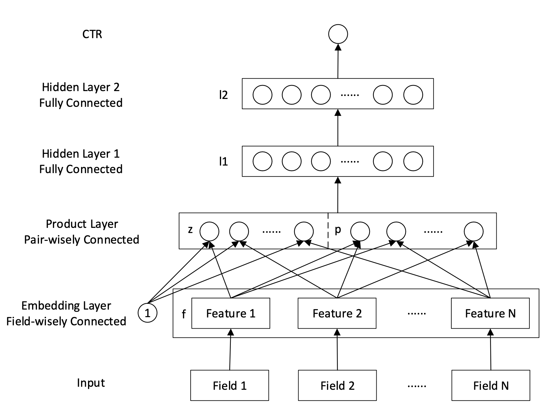
PNN 认为仅用内积(Inner Product)或元素积(Hadamard Product)不足以捕捉所有特征交互信息。因此,它在经典的内积基础上,增加了外积(Outer Product)作为补充,尝试从更丰富的角度来表示特征间的交互 。PNN 的核心创新在于其“乘积层”(Product Layer),该层专门用于对特征 Embedding 进行显式的交叉操作,其输出再送入后续的全连接网络。
PNN 的乘积层会产生两部分信号,一部分是线性信号 l z \mathbf{l}_z l z
l z n = ∑ i = 1 N ∑ k = 1 M ( W z n ) i , k f i k \mathbf{l}_z^n = \sum_{i=1}^N\sum_{k=1}^M (\mathbf{W}_z^n)_{i,k} \mathbf{f}_i^k
l z n = i = 1 ∑ N k = 1 ∑ M ( W z n ) i , k f i k
其中 f i \mathbf{f}_i f i W z n \mathbf{W}_z^n W z n n n n N N N M M M
另一部分是二次信号 l p \mathbf{l}_p l p
IPNN (Inner Product-based Neural Network) : 这种变体使用特征 Embedding 之间的内积 来计算二次信号。一个直接的计算方式是:
l p n = ∑ i = 1 N ∑ j = 1 N ( W p n ) i , j ⟨ f i , f j ⟩ \mathbf{l}_p^n = \sum_{i=1}^N \sum_{j=1}^N (\textbf{W}_p^n)_{i,j} \langle \mathbf{f}_i, \mathbf{f}_j \rangle
l p n = i = 1 ∑ N j = 1 ∑ N ( W p n ) i , j ⟨ f i , f j ⟩
W p n \textbf{W}_p^n W p n n n n O ( N 2 ) O(N^2) O ( N 2 ) N N N W p n \textbf{W}_p^n W p n θ n θ n T \theta_n \theta_n^T θ n θ n T ( W p n ) i , j = θ i , n θ j , n (\textbf{W}_p^n)_{i,j} = \theta_{i,n} \theta_{j,n} ( W p n ) i , j = θ i , n θ j , n
l p n = ∑ i = 1 N ∑ j = 1 N θ i n θ j n ⟨ f i , f j ⟩ = ∑ i = 1 N ∑ j = 1 N ⟨ θ i n f i , θ j n f j ⟩ = ⟨ ∑ i = 1 N θ i n f i , ∑ j = 1 N θ j n f j ⟩ = ∥ ∑ i = 1 N θ i n f i ∥ 2 \mathbf{l}_p^n = \sum_{i=1}^N \sum_{j=1}^N \theta_i^n \theta_j^n \langle \mathbf{f}_i, \mathbf{f}_j \rangle = \sum_{i=1}^N \sum_{j=1}^N \langle \theta_i^n \mathbf{f}_i, \theta_j^n \mathbf{f}_j \rangle = \langle \sum_{i=1}^N \theta_i^n \mathbf{f}_i, \sum_{j=1}^N \theta_j^n \mathbf{f}_j \rangle = \left\|\sum_{i=1}^N \theta_i^n \mathbf{f}_i\right\|^2
l p n = i = 1 ∑ N j = 1 ∑ N θ i n θ j n ⟨ f i , f j ⟩ = i = 1 ∑ N j = 1 ∑ N ⟨ θ i n f i , θ j n f j ⟩ = ⟨ i = 1 ∑ N θ i n f i , j = 1 ∑ N θ j n f j ⟩ = i = 1 ∑ N θ i n f i 2
通过这个变换,计算所有内积对的加权和,转变成了先对 Embedding 进行加权求和,然后计算一次向量的 L2 范数平方 ,复杂度成功地从 O ( N 2 M ) O(N^2M) O ( N 2 M ) O ( N M ) O(NM) O ( NM )
优化后的完整计算公式为:
l p = ( ∥ ∑ i = 1 N θ i 1 f i ∥ 2 , ∥ ∑ i = 1 N θ i 2 f i ∥ 2 , … , ∥ ∑ i = 1 N θ i n f i ∥ 2 ) \mathbf{l}_p = \left(\left\|\sum_{i=1}^N \theta_i^1 \mathbf{f}_i\right\|^2, \left\|\sum_{i=1}^N \theta_i^2 \mathbf{f}_i\right\|^2, \ldots, \left\|\sum_{i=1}^N \theta_i^n \mathbf{f}_i\right\|^2\right)
l p = i = 1 ∑ N θ i 1 f i 2 , i = 1 ∑ N θ i 2 f i 2 , … , i = 1 ∑ N θ i n f i 2
OPNN (Outer Product-based Neural Network) : 这种变体使用特征 Embedding 之间的外积 f i f j T \mathbf{f}_i\mathbf{f}_j^T f i f j T ∑ i = 1 N ∑ j = 1 N f i f j T \sum_{i=1}^N \sum_{j=1}^N \mathbf{f}_i \mathbf{f}_j^T ∑ i = 1 N ∑ j = 1 N f i f j T O ( N 2 M 2 ) O(N^2M^2) O ( N 2 M 2 ) M M M 先将所有特征的 Embedding 向量相加,然后再计算一次外积 :
∑ i = 1 N ∑ j = 1 N f i f j T = ( ∑ i = 1 N f i ) ( ∑ j = 1 N f j ) T \sum_{i=1}^N \sum_{j=1}^N \mathbf{f}_i \mathbf{f}_j^T = (\sum_{i=1}^N \mathbf{f}_i)(\sum_{j=1}^N \mathbf{f}_j)^T
i = 1 ∑ N j = 1 ∑ N f i f j T = ( i = 1 ∑ N f i ) ( j = 1 ∑ N f j ) T
这样,计算量得到了节省 O ( M ( M + N ) ) O(M(M+N)) O ( M ( M + N ))
l p = ( ⟨ W p 1 , ( ∑ i = 1 N f i ) ( ∑ j = 1 N f j ) T ⟩ , ⟨ W p 2 , ( ∑ i = 1 N f i ) ( ∑ j = 1 N f j ) T ⟩ , … , ⟨ W p n , ( ∑ i = 1 N f i ) ( ∑ j = 1 N f j ) T ⟩ ) \mathbf{l}_p = \left(\langle\mathbf{W}_p^1, (\sum_{i=1}^N \mathbf{f}_i)(\sum_{j=1}^N \mathbf{f}_j)^T\rangle, \langle\mathbf{W}_p^2, (\sum_{i=1}^N \mathbf{f}_i)(\sum_{j=1}^N \mathbf{f}_j)^T\rangle, \ldots, \langle\mathbf{W}_p^n, (\sum_{i=1}^N \mathbf{f}_i)(\sum_{j=1}^N \mathbf{f}_j)^T\rangle\right)
l p = ( ⟨ W p 1 , ( i = 1 ∑ N f i ) ( j = 1 ∑ N f j ) T ⟩ , ⟨ W p 2 , ( i = 1 ∑ N f i ) ( j = 1 ∑ N f j ) T ⟩ , … , ⟨ W p n , ( i = 1 ∑ N f i ) ( j = 1 ∑ N f j ) T ⟩ )
其中 对称矩阵W p n ∈ R M × M \mathbf{W}_p^n \in \mathbb{R}^{M \times M} W p n ∈ R M × M n n n ⟨ A , B ⟩ = ∑ i = 1 M ∑ j = 1 M A i , j B i , j \langle \mathbf{A}, \mathbf{B} \rangle = \sum_{i=1}^M \sum_{j=1}^M \mathbf{A}_{i,j} \mathbf{B}_{i,j} ⟨ A , B ⟩ = ∑ i = 1 M ∑ j = 1 M A i , j B i , j
在得到线性信号 l z l_z l z l p l_p l p
l 1 = ReLU ( l z + l p + b 1 ) l 2 = ReLU ( W 2 l 1 + b 2 ) y ^ = σ ( W 3 l 2 + b 3 ) \begin{aligned}
\mathbf{l}_1 &= \text{ReLU}(\mathbf{l}_z + \mathbf{l}_p + \mathbf{b}_1) \\
\mathbf{l}_2 &= \text{ReLU}(\mathbf{W}_2 \mathbf{l}_1 + \mathbf{b}_2) \\
\hat{y} &= \sigma(\textbf{W}_3 \mathbf{l}_2 + b_3)
\end{aligned}
l 1 l 2 y ^ = ReLU ( l z + l p + b 1 ) = ReLU ( W 2 l 1 + b 2 ) = σ ( W 3 l 2 + b 3 )
PNN 的独特之处在于,它将“乘积”操作(无论是内积还是外积)作为了网络中的一个核心计算单元,认为这种操作比传统 DNN 中简单的“加法”操作更能有效地捕捉类别型特征之间的交互关系。
代码
PNN通过内积和外积两种方式计算特征交互。
通过矩阵分解技巧,PNN将内积计算从 O ( N 2 M ) O(N^2M) O ( N 2 M ) O ( N M ) O(NM) O ( NM ) pnn.py 文件:
1
2
3
4
5
6
7
8
9
10
11
12
13
14
15
16
17
18
19
20
21
22
23
24
25
26
27
28
29
30
31
32
33
34
35
36
37
38
39
40
41
42
43
44
45
46
47
48
49
50
51
52
53
54
55
56
57
58
59
60
61
62
63
64
65
66
67
68
69
70
71
72
73
74
75
76
77
78
79
80
81
82
83
84
85
86
87
88
89
import tensorflow as tffrom .utils import ( build_input_layer, build_group_feature_embedding_table_dict, concat_group_embedding, add_tensor_func, get_linear_logits, ) from .layers import DNNs, PNNdef build_pnn_model (feature_columns, model_config ): """ 构建基于乘积的神经网络 (PNN) 排序模型。 Args: feature_columns: FeatureColumn 列表 model_config: 包含参数的字典: - dnn_units: 列表,DNN 隐藏层单元数 (默认 [64, 32]) - product_layer_units: 整数,乘积层输出单元数 (默认 8) - use_inner: 布尔值,是否使用内积 (默认 True) - use_outer: 布尔值,是否使用外积 (默认 True) - use_bn: 布尔值,是否使用批量归一化 (默认 False) - dropout_rate: 浮点数,dropout 率 (默认 0.0) - linear_logits: 布尔值,是否添加线性项 (默认 True) Returns: (model, None, None): 排序模型元组 """ dnn_units = model_config.get("dnn_units" , [64 , 32 ]) product_layer_units = model_config.get("product_layer_units" , 8 ) use_inner = model_config.get("use_inner" , True ) use_outer = model_config.get("use_outer" , True ) use_bn = model_config.get("use_bn" , False ) dropout_rate = model_config.get("dropout_rate" , 0.0 ) linear_logits = model_config.get("linear_logits" , True ) input_layer_dict = build_input_layer(feature_columns) group_embedding_feature_dict = build_group_feature_embedding_table_dict( feature_columns, input_layer_dict, prefix="embedding/" ) interaction_outputs = [] for ( group_feature_name, group_feature_embedding, ) in group_embedding_feature_dict.items(): if group_feature_name.startswith("pnn" ): pnn_out = PNN( units=product_layer_units, use_inner=use_inner, use_outer=use_outer )(group_feature_embedding) interaction_outputs.append(pnn_out) if len (interaction_outputs) > 1 : interaction_outputs = tf.concat(interaction_outputs, axis=-1 ) else : interaction_outputs = interaction_outputs[0 ] dnn_out = DNNs( units=dnn_units, activation="relu" , use_bn=use_bn, dropout_rate=dropout_rate )(interaction_outputs) pnn_logits = tf.keras.layers.Dense(1 , activation=None )(dnn_out) if linear_logits: linear_logit = get_linear_logits(input_layer_dict, feature_columns) pnn_logits = add_tensor_func( [pnn_logits, linear_logit], name="pnn_linear_logits" ) pnn_logits = tf.keras.layers.Flatten()(pnn_logits) output = tf.keras.layers.Dense(1 , activation="sigmoid" , name="pnn_output" )( pnn_logits ) output = tf.keras.layers.Flatten()(output) model = tf.keras.models.Model( inputs=list (input_layer_dict.values()), outputs=output ) return model, None , None
1.5 FiBiNET: 特征重要性与双线性交互
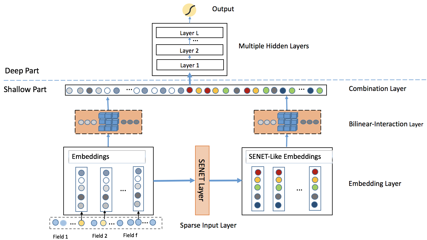
虽然 PNN 通过内积和外积丰富了特征交互的表达方式,但它仍然将所有特征视为同等重要。然而,在实际的推荐场景中,不同特征对于预测结果的贡献度显然是不同的。FiBiNET (Feature Importance and Bilinear feature Interaction Network) 模型认识到了这个问题,它在进行二阶特征交叉之前,先动态地学习每个特征的重要性权重,然后再通过双线性交互来捕捉更精细的特征关系 。这种设计使得模型能够有选择性地进行特征交互,从而提升二阶特征交叉的质量。
FiBiNET 的创新主要体现在两个核心模块上:SENET 特征重要性学习机制 和双线性交互层 。
SENET 特征重要性学习
FiBiNET 引入了来自计算机视觉领域的 SENET (Squeeze-and-Excitation Network) 机制,用于动态学习每个特征的重要性权重。与传统方法对所有特征一视同仁不同,SENET 能够自适应地为不同特征分配不同的权重,让模型更加关注那些对预测任务更重要的特征。
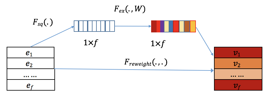
SENET 的工作流程包含三个关键步骤:
Squeeze (挤压) : 通过全局平均池化将每个特征的 k k k e i \mathbf{e}_i e i
z i = F sq ( e i ) = 1 k ∑ t = 1 k e i ( t ) \mathbf{z}_i = F_{\text{sq}}(\mathbf{e}_i) = \frac{1}{k} \sum_{t=1}^k \mathbf{e}_i(t)
z i = F sq ( e i ) = k 1 t = 1 ∑ k e i ( t )
Excitation (激励) : 使用两个全连接层构成的瓶颈结构来学习特征间的相关性,并生成每个特征的重要性权重:
A = F ex ( Z ) = σ 2 ( W 2 σ 1 ( W 1 Z ) ) \mathbf{A} = F_{\text{ex}}(\mathbf{Z}) = \sigma_2(\mathbf{W}_2 \sigma_1(\mathbf{W}_1 \mathbf{Z}))
A = F ex ( Z ) = σ 2 ( W 2 σ 1 ( W 1 Z ))
其中 W 1 ∈ R f × f r \mathbf{W}_1 \in \mathbb{R}^{f \times \frac{f}{r}} W 1 ∈ R f × r f W 2 ∈ R f r × f \mathbf{W}_2 \in \mathbb{R}^{\frac{f}{r} \times f} W 2 ∈ R r f × f r r r
Re-weight (重新加权) : 将学习到的权重应用于原始嵌入向量:
V = F ReWeight ( A , E ) = [ a 1 ⋅ e 1 , a 2 ⋅ e 2 , … , a f ⋅ e f ] \mathbf{V} = F_{\text{ReWeight}}(\mathbf{A}, \mathbf{E}) = [\mathbf{a}_1 \cdot \mathbf{e}_1, \mathbf{a}_2 \cdot \mathbf{e}_2, \ldots, \mathbf{a}_f \cdot \mathbf{e}_f]
V = F ReWeight ( A , E ) = [ a 1 ⋅ e 1 , a 2 ⋅ e 2 , … , a f ⋅ e f ]
双线性交互层
在获得原始嵌入 E \mathbf{E} E V \mathbf{V} V W ∈ R k × k \mathbf{W} \in \mathbb{R}^{k \times k} W ∈ R k × k
p i j = v i ⋅ W ∘ v j \mathbf{p}_{ij} = \mathbf{v}_i \cdot \mathbf{W} \circ \mathbf{v}_j
p ij = v i ⋅ W ∘ v j
其中 ∘ \circ ∘
FiBiNET 会同时对原始嵌入 E \mathbf{E} E V \mathbf{V} V FiBiNET 不仅解决了"哪些特征更重要"的问题,还通过双线性交互提升了二阶特征交叉的表达能力 。
代码
FiBiNET的实现包含两个关键部分:SENET特征重要性学习和双线性交互。
FiBiNET通过SENET动态调整特征重要性,通过双线性变换增强特征交互的表达能力,相比传统方法更加灵活和高效。fibinet.py 文件:
1
2
3
4
5
6
7
8
9
10
11
12
13
14
15
16
17
18
19
20
21
22
23
24
25
26
27
28
29
30
31
32
33
34
35
36
37
38
39
40
41
42
43
44
45
46
47
48
49
50
51
52
53
54
55
56
57
58
59
60
61
62
63
64
65
66
67
68
69
70
71
72
73
74
75
76
77
78
79
80
81
82
83
84
85
86
87
88
89
90
91
92
93
94
95
96
97
98
99
100
101
102
103
104
105
106
107
108
import tensorflow as tffrom .utils import ( build_input_layer, build_group_feature_embedding_table_dict, concat_group_embedding, add_tensor_func, get_linear_logits, ) from .layers import DNNs, SENetLayer, BilinearInteractionLayerdef build_fibinet_model (feature_columns, model_config ): """ 构建 FiBiNET(特征重要性和双线性特征交互网络)排序模型。 Args: feature_columns: FeatureColumn 列表 model_config: 包含参数的字典: - dnn_units: list,DNN 隐藏层单元数(默认 [64, 32]) - senet_reduction_ratio: int,SENet 压缩比例(默认 3) - bilinear_type: str,双线性交互类型(默认 "interaction") - use_bn: bool,是否使用批归一化(默认 False) - dropout_rate: float,dropout 比例(默认 0.0) - linear_logits: bool,是否添加线性项(默认 True) Returns: (model, None, None): 排序模型元组 """ dnn_units = model_config.get("dnn_units" , [64 , 32 ]) senet_reduction_ratio = model_config.get("senet_reduction_ratio" , 3 ) bilinear_type = model_config.get("bilinear_type" , "interaction" ) use_bn = model_config.get("use_bn" , False ) dropout_rate = model_config.get("dropout_rate" , 0.0 ) linear_logits = model_config.get("linear_logits" , True ) input_layer_dict = build_input_layer(feature_columns) group_embedding_feature_dict = build_group_feature_embedding_table_dict( feature_columns, input_layer_dict, prefix="embedding/" ) interaction_outputs = [] for ( group_feature_name, group_feature_embedding, ) in group_embedding_feature_dict.items(): if group_feature_name.startswith("fibinet" ): group_feature = concat_group_embedding( group_embedding_feature_dict, group_feature_name, axis=1 , flatten=False ) senet_enhanced_features = SENetLayer(reduction_ratio=senet_reduction_ratio)( group_feature ) bilinear_interaction = BilinearInteractionLayer( bilinear_type=bilinear_type )(group_feature) bilinear_senet_interaction = BilinearInteractionLayer( bilinear_type=bilinear_type )(senet_enhanced_features) bilinear_flat = tf.keras.layers.Flatten()(bilinear_interaction) bilinear_senet_flat = tf.keras.layers.Flatten()(bilinear_senet_interaction) interaction_outputs.extend([bilinear_flat, bilinear_senet_flat]) if len (interaction_outputs) > 1 : interaction_outputs = tf.concat(interaction_outputs, axis=-1 ) else : interaction_outputs = interaction_outputs[0 ] dnn_out = DNNs( units=dnn_units, activation="relu" , use_bn=use_bn, dropout_rate=dropout_rate )(interaction_outputs) fibinet_logits = tf.keras.layers.Dense(1 , activation=None )(dnn_out) if linear_logits: linear_logit = get_linear_logits(input_layer_dict, feature_columns) fibinet_logits = add_tensor_func( [fibinet_logits, linear_logit], name="fibinet_linear_logits" ) fibinet_logits = tf.keras.layers.Flatten()(fibinet_logits) output = tf.keras.layers.Dense(1 , activation="sigmoid" , name="fibinet_output" )( fibinet_logits ) output = tf.keras.layers.Flatten()(output) model = tf.keras.models.Model( inputs=list (input_layer_dict.values()), outputs=output ) return model, None , None
1.6 DeepFM: 低阶高阶的统一建模
原理
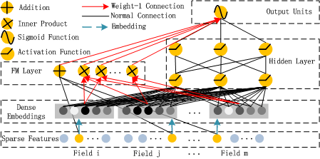
DeepFM 是对 Wide & Deep 架构的直接改进和优化。它将 Wide & Deep 中需要大量人工特征工程的 Wide 部分,直接替换为了一个无需任何人工干预的 FM 模型 ,从而实现了真正的端到端训练。更关键的是,DeepFM 中的 FM 组件和 Deep 组件共享同一份特征嵌入(Embedding) ,这带来了两大好处:首先,模型可以同时从原始特征中学习低阶和高阶的特征交互;其次,共享 Embedding 的方式使得模型训练更加高效。
DeepFM 的结构非常清晰,它由 FM 和 DNN 两个并行的组件构成,两者共享输入。
FM 组件 : 负责学习一阶特征和二阶特征交叉。其输出 yFM 的计算方式与标准 FM 完全相同:
y F M = ⟨ w , x ⟩ + ∑ i = 1 d ∑ j = i + 1 d ⟨ V i , V j ⟩ x i x j y_{FM} = \langle w, x \rangle + \sum_{i=1}^d \sum_{j=i+1}^d \langle V_{i}, V_{j} \rangle x_{i}x_{j}
y FM = ⟨ w , x ⟩ + i = 1 ∑ d j = i + 1 ∑ d ⟨ V i , V j ⟩ x i x j
这里的 V i V_{i} V i i i i
Deep 组件 : 负责学习高阶的非线性特征交叉。它的输入正是 FM 组件中所使用的那一套 Embedding 向量。具体来说,所有输入特征首先被映射到它们的低维 Embedding 向量上,然后这些 Embedding 向量被拼接(concatenate)在一起,形成一个长的向量,作为 DNN 的输入。
a ( 0 ) = [ e 1 , e 2 , . . . , e m ] a^{(0)} = [e_1, e_2, ..., e_m]
a ( 0 ) = [ e 1 , e 2 , ... , e m ]
其中 e i e_i e i i i i
a ( l + 1 ) = σ ( W ( l ) a ( l ) + b ( l ) ) a^{(l+1)} = \sigma(\textbf{W}^{(l)} a^{(l)} + \textbf{b}^{(l)})
a ( l + 1 ) = σ ( W ( l ) a ( l ) + b ( l ) )
其中 l l l σ \sigma σ W ( l ) \textbf{W}^{(l)} W ( l ) b ( l ) \textbf{b}^{(l)} b ( l ) l l l
y D e e p = W ∣ H ∣ + 1 ⋅ a ∣ H ∣ + b ∣ H ∣ + 1 y_{Deep} = \textbf{W}^{|H|+1} \cdot a^{|H|} + \textbf{b}^{|H|+1}
y Dee p = W ∣ H ∣ + 1 ⋅ a ∣ H ∣ + b ∣ H ∣ + 1
其中 H H H
最终,DeepFM 的总输出是 FM 部分和 Deep 部分输出的简单相加,再通过一个 Sigmoid 函数得到最终的点击率预测值:
y ^ = σ ( y F M + y D e e p ) \hat{y} = \sigma(y_{FM} + y_{Deep})
y ^ = σ ( y FM + y Dee p )
DeepFM模型成功地结合了FM的低阶特征学习能力和深度神经网络的高阶特征学习能力。通过FM组件和深度组件共享相同的特征嵌入,模型可以同时从原始特征中学习低阶和高阶特征交互,无需像Wide & Deep那样依赖专家的特征工程。这种设计使得DeepFM成为一个端到端的自动特征学习模型,在效果和效率上都表现出色。
代码
DeepFM的关键在于FM和DNN两个组件共享同一套Embedding,各自负责不同层次的特征交互。
DeepFM通过共享Embedding实现了端到端训练,FM组件捕捉低阶交叉,DNN组件学习高阶模式,两者互补形成高效的特征学习能力。deepfm.py 文件:
1
2
3
4
5
6
7
8
9
10
11
12
13
14
15
16
17
18
19
20
21
22
23
24
25
26
27
28
29
30
31
32
33
34
35
36
37
38
39
40
41
42
43
44
45
46
47
48
49
50
51
52
53
54
55
56
57
58
59
60
61
62
63
64
65
66
67
68
69
70
71
72
73
74
75
76
77
78
79
80
81
82
83
84
85
86
87
88
89
90
91
92
93
94
95
import tensorflow as tffrom .utils import ( build_input_layer, build_group_feature_embedding_table_dict, concat_group_embedding, add_tensor_func, get_linear_logits, ) from .layers import FM, DNNsdef build_deepfm_model (feature_columns, model_config ): """ 构建 DeepFM (深度分解机) 排序模型。 参数: feature_columns: FeatureColumn 列表 model_config: 包含以下参数的字典: - dnn_units: list, DNN 隐藏层单元数 (默认 [64, 32]) - dropout_rate: float, dropout 率 (默认 0.1) - linear_logits: bool, 是否添加线性项 (默认 True) 返回: (model, None, None): 排序模型元组 """ dnn_units = model_config.get("dnn_units" , [64 , 32 ]) dropout_rate = model_config.get("dropout_rate" , 0.1 ) linear_logits = model_config.get("linear_logits" , True ) input_layer_dict = build_input_layer(feature_columns) group_embedding_feature_dict = build_group_feature_embedding_table_dict( feature_columns, input_layer_dict, prefix="embedding/" ) fm_outputs = [] dnn_outputs = [] for ( group_feature_name, group_feature_embedding, ) in group_embedding_feature_dict.items(): if group_feature_name.startswith("deepfm" ): concat_feature = concat_group_embedding( group_embedding_feature_dict, group_feature_name, axis=1 , flatten=False ) fm_out = FM(name=f"fm_{group_feature_name} " )(concat_feature) fm_outputs.append(fm_out) flatten_feature = tf.keras.layers.Flatten()(concat_feature) dnn_out = DNNs( name=f"dnn_{group_feature_name} " , units=dnn_units + [1 ], dropout_rate=dropout_rate, )(flatten_feature) dnn_outputs.append(dnn_out) if len (fm_outputs) > 1 : fm_logit = add_tensor_func(fm_outputs, name="fm_logits" ) else : fm_logit = fm_outputs[0 ] if len (dnn_outputs) > 1 : dnn_logit = add_tensor_func(dnn_outputs, name="dnn_logits" ) else : dnn_logit = dnn_outputs[0 ] if linear_logits: linear_logit = get_linear_logits(input_layer_dict, feature_columns) fm_logit = add_tensor_func([fm_logit, linear_logit], name="fm_linear_logits" ) deepfm_logits = add_tensor_func([fm_logit, dnn_logit], name="deepfm_logits" ) deepfm_logits = tf.keras.layers.Flatten()(deepfm_logits) output = tf.keras.layers.Dense(1 , activation="sigmoid" , name="deepfm_output" )( deepfm_logits ) output = tf.keras.layers.Flatten()(output) model = tf.keras.models.Model( inputs=list (input_layer_dict.values()), outputs=output ) return model, None , None
2、高阶特征交叉
前面我们学了各种二阶特征交叉技术,这些模型能够明确地处理二阶交互,但对于更高阶的特征组合,它们主要靠深度神经网络来学习。深度网络虽然能学到高阶交互,但我们不知道它具体学到了什么,也不清楚这些交互是怎么影响预测的。所以研究者们想:能不能像 FM 处理二阶交叉那样,设计出能够明确捕捉高阶交叉的网络结构?
2.1 DCN: 残差连接的高阶交叉
原理
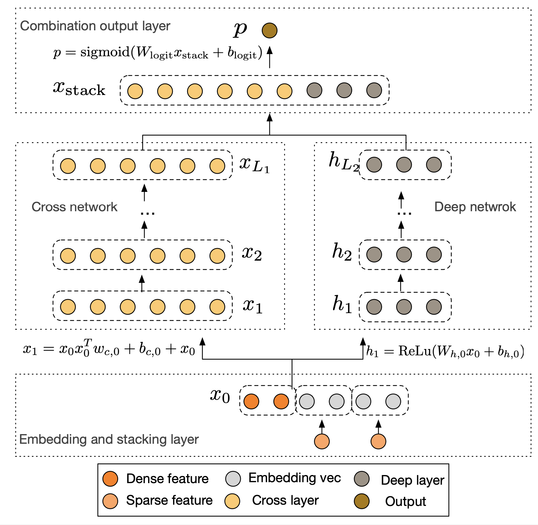
为了解决上述问题,Deep & Cross Network (DCN) 通过一个创新的Cross Network来替代Wide & Deep模型中的Wide部分。该网络的核心思想是在每一层都与原始的输入特征进行交叉,从而以一种显式且可控的方式,自动构建更高阶的特征交互,而无需繁琐的人工特征工程。
DCN的整体结构由并行的Cross Network和Deep Network两部分组成,它们共享相同的Embedding层输入。首先,模型将稀疏的类别特征转换为低维稠密的Embedding向量,并与数值型特征拼接在一起,形成统一的输入向量 x 0 \mathbf{x}_0 x 0
x 0 = [ x embed , 1 T , … , x embed , k T , x dense T ] \mathbf{x}_0 = [\mathbf{x}_{\text{embed}, 1}^T, \ldots, \mathbf{x}_{\text{embed}, k}^T, \mathbf{x}_{\text{dense}}^T]
x 0 = [ x embed , 1 T , … , x embed , k T , x dense T ]
这个初始向量 x 0 \mathbf{x}_0 x 0
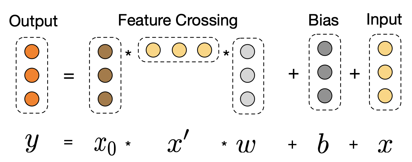
Cross Network是DCN的核心创新。它由多个交叉层堆叠而成,其精妙之处在于每一层的计算都保留了与原始输入 x 0 \mathbf{x}_0 x 0 l + 1 l+1 l + 1
x l + 1 = x 0 x l T w l + b l + x l \mathbf{x}_{l+1} = \mathbf{x}_0 \mathbf{x}_l^T \mathbf{w}_l + \mathbf{b}_l + \mathbf{x}_l
x l + 1 = x 0 x l T w l + b l + x l
其中x l , x l + 1 ∈ R d \mathbf{x}_l, \mathbf{x}_{l+1} \in \mathbb{R}^d x l , x l + 1 ∈ R d l l l l + 1 l+1 l + 1 x 0 ∈ R d \mathbf{x}_0 \in \mathbb{R}^d x 0 ∈ R d w l , b l ∈ R d \mathbf{w}_l, \mathbf{b}_l \in \mathbb{R}^d w l , b l ∈ R d l l l
我们可以观察到,这个结构本质上是一个残差网络。每一层都在上一层输出 x l \mathbf{x}_l x l x 0 x l T w l \mathbf{x}_0 \mathbf{x}_l^T \mathbf{w}_l x 0 x l T w l b l \mathbf{b}_l b l x 0 \mathbf{x}_0 x 0 x l \mathbf{x}_l x l 特征交叉的阶数也随之增加 。例如,在第一层(l = 0 l=0 l = 0 x 1 \mathbf{x}_1 x 1 x 0 \mathbf{x}_0 x 0 l = 1 l=1 l = 1 x 1 \mathbf{x}_1 x 1 x 0 \mathbf{x}_0 x 0
与Cross Network并行的Deep Network部分是一个标准的全连接神经网络,用于隐式地学习高阶非线性关系,其结构与我们熟悉的DeepFM中的DNN部分类似。最后,模型将Cross Network的输出 x L 1 \mathbf{x}_{L_1} x L 1 h L 2 \mathbf{h}_{L_2} h L 2
p = σ ( [ x L 1 T , h L 2 T ] w logits ) \mathbf{p} = \sigma([\mathbf{x}_{L_1}^T, \mathbf{h}_{L_2}^T] \mathbf{w}_{\text{logits}})
p = σ ([ x L 1 T , h L 2 T ] w logits )
DCN通过Cross Network提供了一种有效且高效的显式高阶特征交叉方案,并结合DNN的隐式交叉能力,为推荐模型的设计提供了新的思路。
代码
DCN的核心在于Cross Network的交叉层计算。每一层都保持与原始输入 x 0 x_0 x 0
这个设计的巧妙之处在于:通过残差连接保留了原始信息,通过与 x 0 x_0 x 0 dcn.py 文件:
1
2
3
4
5
6
7
8
9
10
11
12
13
14
15
16
17
18
19
20
21
22
23
24
25
26
27
28
29
30
31
32
33
34
35
36
37
38
39
40
41
42
43
44
45
46
47
48
49
50
51
52
53
54
55
56
57
58
59
60
61
62
63
64
65
66
67
68
69
70
71
72
73
74
75
76
77
78
79
80
81
82
83
84
85
86
87
88
89
90
91
92
93
94
95
96
97
98
99
100
101
102
103
104
105
106
107
108
109
110
111
112
113
114
115
116
117
118
119
import tensorflow as tffrom .utils import ( build_input_layer, build_group_feature_embedding_table_dict, concat_group_embedding, add_tensor_func, get_linear_logits, ) from .layers import DNNs, DCNdef build_dcn_model (feature_columns, model_config ): """ 构建 DCN (深度交叉网络) 排序模型。 参数: feature_columns: FeatureColumn 列表 model_config: 包含以下参数的字典: - num_cross_layers: int, 交叉层数量 (默认 3) - dnn_units: list, DNN 隐藏单元 (默认 [64, 32]) - dropout_rate: float, dropout 率 (默认 0.1) - l2_reg: float, L2 正则化 (默认 1e-5) - linear_logits: bool, 是否添加线性项 (默认 True) 返回: (model, None, None): 排序模型元组 """ num_cross_layers = model_config.get("num_cross_layers" , 3 ) dnn_units = model_config.get("dnn_units" , [64 , 32 ]) dropout_rate = model_config.get("dropout_rate" , 0.1 ) l2_reg = model_config.get("l2_reg" , 1e-5 ) linear_logits = model_config.get("linear_logits" , True ) input_layer_dict = build_input_layer(feature_columns) group_embedding_feature_dict = build_group_feature_embedding_table_dict( feature_columns, input_layer_dict, prefix="embedding/" ) cross_outputs = [] deep_outputs = [] for ( group_feature_name, group_feature_embedding, ) in group_embedding_feature_dict.items(): if group_feature_name.startswith("dcn" ): concat_feature = concat_group_embedding( group_embedding_feature_dict, group_feature_name, axis=-1 , flatten=True ) cross_out = DCN(num_cross_layers=num_cross_layers, l2_reg=l2_reg)( concat_feature ) cross_outputs.append(cross_out) elif group_feature_name.startswith("dnn" ): concat_feature = concat_group_embedding( group_embedding_feature_dict, group_feature_name, axis=-1 , flatten=True ) dnn_out = DNNs( units=dnn_units, dropout_rate=dropout_rate, activation="relu" , use_bn=False , )(concat_feature) deep_outputs.append(dnn_out) if len (cross_outputs) > 1 : cross_logit = add_tensor_func(cross_outputs, name="cross_logits" ) else : cross_logit = cross_outputs[0 ] if cross_outputs else None if len (deep_outputs) > 1 : deep_logit = add_tensor_func(deep_outputs, name="dnn_logits" ) else : deep_logit = deep_outputs[0 ] if deep_outputs else None dcn_outputs = [] if cross_logit is not None : dcn_outputs.append(cross_logit) if deep_logit is not None : dcn_outputs.append(deep_logit) if len (dcn_outputs) > 1 : dcn_logits = tf.keras.layers.Concatenate(name="dcn_concat" )(dcn_outputs) else : dcn_logits = dcn_outputs[0 ] if linear_logits: linear_logit = get_linear_logits(input_layer_dict, feature_columns) dcn_logits = tf.keras.layers.Dense(1 , name="dcn_dense" )(dcn_logits) dcn_logits = add_tensor_func( [dcn_logits, linear_logit], name="dcn_linear_logits" ) else : dcn_logits = tf.keras.layers.Dense(1 , name="dcn_dense" )(dcn_logits) dcn_logits = tf.keras.layers.Flatten()(dcn_logits) output = tf.keras.layers.Dense(1 , activation="sigmoid" , name="dcn_output" )( dcn_logits ) output = tf.keras.layers.Flatten()(output) model = tf.keras.models.Model( inputs=list (input_layer_dict.values()), outputs=output ) return model, None , None
2.2 xDeepFM: 向量级别的特征交互
原理
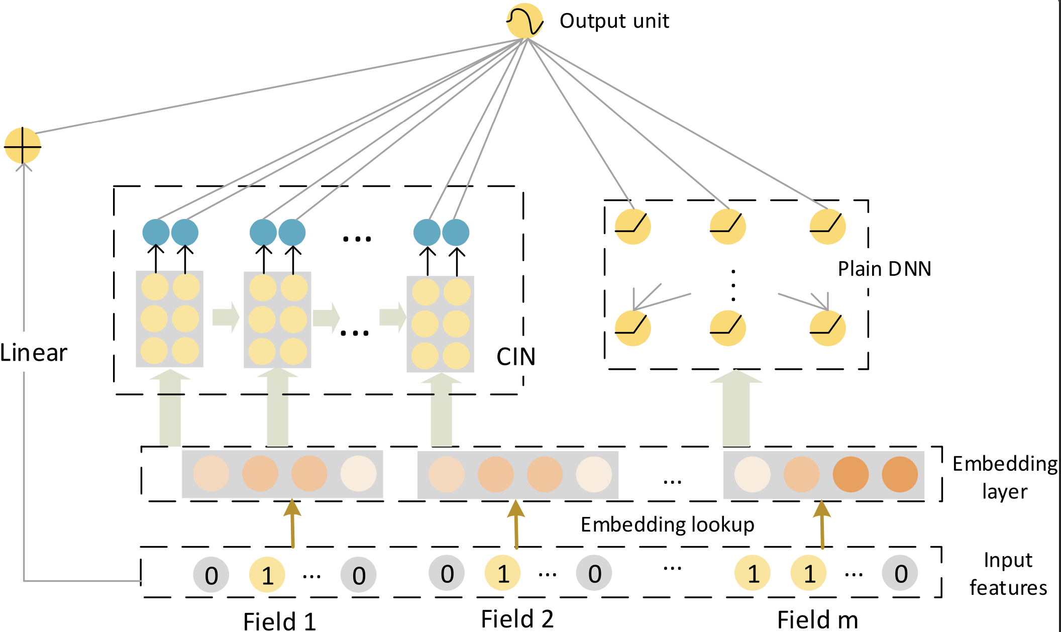
尽管DCN能够显式地构建高阶特征,但它的交叉方式是在 元素级别(bit-wise) 上进行的。这意味着Embedding向量中的每一个元素都会独立地与其他特征的Embedding元素进行交互,这在一定程度上忽略了Embedding向量作为一个整体所代表的特征场的概念。为了解决这个问题,xDeepFM模型被提了出来,其核心是设计了一个全新的压缩交互网络(Compressed Interaction Network, CIN) ,以 向量级别(vector-wise) 的方式进行特征交互,这更符合我们进行特征工程时的直觉。
xDeepFM的整体架构同样由三部分组成:一个传统的线性部分、一个用于隐式高阶交叉的DNN,以及创新的CIN网络用于显式高阶交叉。这三部分的输出最终被结合起来进行预测。
CIN的设计目标是实现向量级别的显式高阶交互,同时控制网络复杂度。它的输入是一个m × D m \times D m × D X 0 \mathbf{X}_0 X 0 m m m D D D i i i i i i e i \mathbf{e}_i e i
CIN的计算过程在每一层都分为两步。在计算第 k k k X k \mathbf{X}_k X k X k − 1 \mathbf{X}_{k-1} X k − 1 X 0 \mathbf{X}_0 X 0
第一步,模型计算出上一层输出的 H k − 1 H_{k-1} H k − 1 m m m ∘ \circ ∘ H k − 1 × m H_{k-1} \times m H k − 1 × m D D D
第二步,为了生成第 k k k h h h X h , ∗ k \mathbf{X}_{h,*}^k X h , ∗ k
综合起来,其核心计算公式如下:
X h , ∗ k = ∑ i = 1 H k − 1 ∑ j = 1 m W i , j k , h ( X i , ∗ k − 1 ∘ X j , ∗ 0 ) \mathbf{X}_{h,*}^k = \sum_{i=1}^{H_{k-1}} \sum_{j=1}^{m} \mathbf{W}_{i,j}^{k,h} (\mathbf{X}_{i,*}^{k-1} \circ \mathbf{X}_{j,*}^0)
X h , ∗ k = i = 1 ∑ H k − 1 j = 1 ∑ m W i , j k , h ( X i , ∗ k − 1 ∘ X j , ∗ 0 )
其中:
X k ∈ R H k × D \mathbf{X}_k \in \mathbb{R}^{H_k \times D} X k ∈ R H k × D k k k H k H_k H k H k H_k H k k k k
X i , ∗ k − 1 \mathbf{X}_{i,*}^{k-1} X i , ∗ k − 1 k − 1 k-1 k − 1 i i i D D D
X j , ∗ 0 \mathbf{X}_{j,*}^0 X j , ∗ 0 j j j D D D j j j
∘ \circ ∘ 向量级别的交互 ,保留了 D D D
W k , h ∈ R H k − 1 × m \mathbf{W}_{k,h} \in \mathbb{R}^{H_{k-1} \times m} W k , h ∈ R H k − 1 × m ( X i , ∗ k − 1 , X j , ∗ 0 ) (\mathbf{X}_{i,*}^{k-1}, \mathbf{X}_{j,*}^0) ( X i , ∗ k − 1 , X j , ∗ 0 ) H k − 1 × m H_{k-1} \times m H k − 1 × m D D D X h , ∗ k \mathbf{X}_{h,*}^k X h , ∗ k
这个过程清晰地展示了特征交互是如何在向量级别上逐层发生的。第 k k k X k \mathbf{X}_k X k k + 1 k+1 k + 1
在计算出每一层(从第1 1 1 T T T X k \mathbf{X}_k X k X k \mathbf{X}_k X k H k H_k H k D D D p k ∈ R H k \mathbf{p}_k \in \mathbb{R}^{H_k} p k ∈ R H k
p + = [ p 1 , p 2 , … , p T ] \mathbf{p}^+ = [\mathbf{p}_1, \mathbf{p}_2, \ldots, \mathbf{p}_T]
p + = [ p 1 , p 2 , … , p T ]
这个输出 p + \mathbf{p}^+ p + T + 1 T+1 T + 1
y ^ = σ ( w linear T a + w dnn T x dnn k + w cin T p + + b ) \hat{y} = \sigma(\mathbf{w}_{\text{linear}}^T \mathbf{a} + \mathbf{w}_{\text{dnn}}^T \mathbf{x}_{\text{dnn}}^k + \mathbf{w}_{\text{cin}}^T \mathbf{p}^+ + \mathbf{b})
y ^ = σ ( w linear T a + w dnn T x dnn k + w cin T p + + b )
其中a \mathbf{a} a x dnn k \mathbf{x}_{\text{dnn}}^k x dnn k b \mathbf{b} b
通过引入CIN,xDeepFM成功地将显性的、向量级别的特征交互与隐性的、元素级别的特征交互结合在同一个模型中 ,为自动学习高阶特征交互提供了又一个强大且更具解释性的解决方案。
代码
CIN的核心在于向量级别的特征交互计算。每一层都通过哈达玛积实现上一层输出与原始输入的交叉。
CIN通过保持向量结构的交互方式,既实现了显式的高阶特征组合,又避免了参数量的过快增长。xdeepfm.py 文件:
1
2
3
4
5
6
7
8
9
10
11
12
13
14
15
16
17
18
19
20
21
22
23
24
25
26
27
28
29
30
31
32
33
34
35
36
37
38
39
40
41
42
43
44
45
46
47
48
49
50
51
52
53
54
55
56
57
58
59
60
61
62
63
64
65
66
67
68
69
70
71
72
73
74
75
76
77
78
79
80
81
82
83
84
85
86
87
88
89
90
91
92
93
94
95
96
97
98
99
100
101
102
103
104
105
106
107
108
109
110
111
112
113
114
115
116
import tensorflow as tffrom .utils import ( build_input_layer, build_group_feature_embedding_table_dict, concat_group_embedding, add_tensor_func, get_linear_logits, ) from .layers import DNNs, CINsdef build_xdeepfm_model (feature_columns, model_config ): """ 构建 xDeepFM (极端深度因子分解机) 排序模型。 Args: feature_columns: FeatureColumn 列表 model_config: 包含参数的字典: - dnn_units: 列表,DNN 隐藏层单元数 (默认 [64, 32]) - dnn_dropout_rate: 浮点数,DNN 的 dropout 率 (默认 0.1) - cin_layer_sizes: 列表,CIN 层大小 (默认 [32, 16]) - l2_reg: 浮点数,L2 正则化 (默认 1e-5) - linear_logits: 布尔值,是否添加线性项 (默认 True) Returns: (model, None, None): 排序模型元组 """ dnn_units = model_config.get("dnn_units" , [64 , 32 ]) dnn_dropout_rate = model_config.get("dnn_dropout_rate" , 0.1 ) cin_layer_sizes = model_config.get("cin_layer_sizes" , [32 , 16 ]) l2_reg = model_config.get("l2_reg" , 1e-5 ) linear_logits = model_config.get("linear_logits" , True ) input_layer_dict = build_input_layer(feature_columns) group_embedding_feature_dict = build_group_feature_embedding_table_dict( feature_columns, input_layer_dict, prefix="embedding/" ) dnn_logits = [] cin_logits = [] for ( group_feature_name, group_feature_embedding, ) in group_embedding_feature_dict.items(): if group_feature_name.startswith("xdeepfm" ): concat_feature = concat_group_embedding( group_embedding_feature_dict, group_feature_name, axis=1 , flatten=False ) flatten_feature = tf.keras.layers.Flatten()(concat_feature) dnn_out = DNNs( units=dnn_units, dropout_rate=dnn_dropout_rate, activation="relu" , use_bn=False , )(flatten_feature) dnn_logit = tf.keras.layers.Dense( 1 , activation=None , name=f"dnn_{group_feature_name} " )(dnn_out) dnn_logits.append(dnn_logit) cin_out = CINs(cin_layer_sizes, l2_reg=l2_reg)(concat_feature) cin_logit = tf.keras.layers.Dense( 1 , activation=None , name=f"cin_{group_feature_name} " )(cin_out) cin_logits.append(cin_logit) if len (dnn_logits) > 1 : dnn_combined = add_tensor_func(dnn_logits, name="dnn_logits" ) else : dnn_combined = dnn_logits[0 ] if dnn_logits else None if len (cin_logits) > 1 : cin_combined = add_tensor_func(cin_logits, name="cin_logits" ) else : cin_combined = cin_logits[0 ] if cin_logits else None xdeepfm_outputs = [] if dnn_combined is not None : xdeepfm_outputs.append(dnn_combined) if cin_combined is not None : xdeepfm_outputs.append(cin_combined) if linear_logits: linear_logit = get_linear_logits(input_layer_dict, feature_columns) xdeepfm_outputs.append(linear_logit) if len (xdeepfm_outputs) > 1 : xdeepfm_logits = add_tensor_func(xdeepfm_outputs, name="xdeepfm_logits" ) else : xdeepfm_logits = xdeepfm_outputs[0 ] xdeepfm_logits = tf.keras.layers.Flatten()(xdeepfm_logits) output = tf.keras.layers.Dense(1 , activation="sigmoid" , name="xdeepfm_output" )( xdeepfm_logits ) output = tf.keras.layers.Flatten()(output) model = tf.keras.models.Model( inputs=list (input_layer_dict.values()), outputs=output ) return model, None , None
2.3 AutoInt: 自注意力的自适应交互
DCN通过残差连接实现了元素级别的高阶交互,xDeepFM通过CIN网络实现了向量级别的高阶交互,但这两种方法都有一个共同的局限性:它们对高阶特征交互的构建方式是相对固定的。DCN的每一层都必须与原始输入进行交叉,而xDeepFM的CIN网络则按照预定义的方式进行向量交互。那么,能否设计一种更加灵活、智能的高阶特征交互机制,让模型自主地决定哪些特征应该参与交互,以及交互的强度如何?
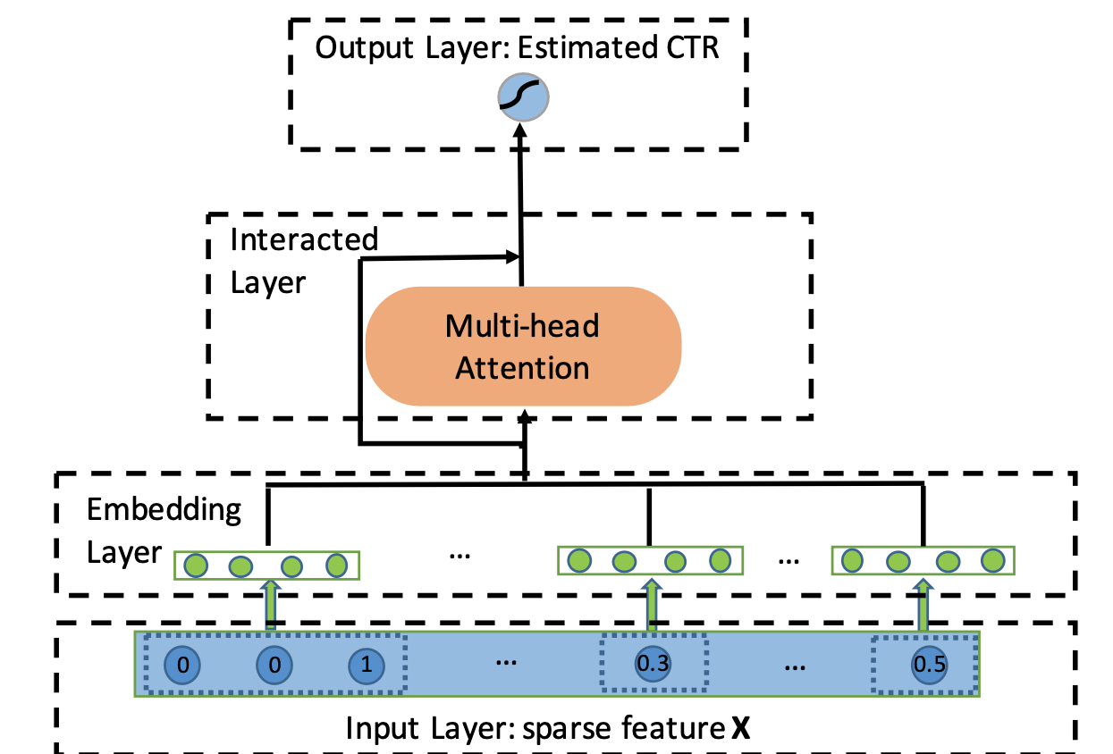
AutoInt (Automatic Feature Interaction) 模型回答了这个问题。它借鉴了自然语言处理领域中 Transformer 架构的核心思想,通过多头自注意力机制来自动、自适应地学习任意阶数的特征交互 。与前面介绍的方法不同,AutoInt 不依赖于固定的交互模式,而是让模型在训练过程中学习出最有效的特征交互组合。
AutoInt 的整体架构相对简洁,它将所有输入特征(无论是类别型还是数值型)都转换为相同维度的嵌入向量 e m ∈ R d \mathbf{e}_m \in \mathbb{R}^d e m ∈ R d m m m m m m
多头自注意力机制
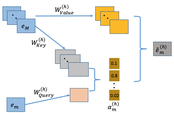
AutoInt 的核心是其交互层,该层由多头自注意力机制构成。对于任意两个特征的嵌入向量 e m \mathbf{e}_m e m e k \mathbf{e}_k e k h h h m m m k k k h h h α m , k ( h ) \alpha_{m,k}^{(h)} α m , k ( h )
α m , k ( h ) = exp ( ψ ( h ) ( e m , e k ) ) ∑ l = 1 M exp ( ψ ( h ) ( e m , e l ) ) \alpha_{m,k}^{(h)} = \frac{\exp(\psi^{(h)}(\mathbf{e}_m, \mathbf{e}_k))}{\sum_{l=1}^{M}\exp(\psi^{(h)}(\mathbf{e}_m, \mathbf{e}_l))}
α m , k ( h ) = ∑ l = 1 M exp ( ψ ( h ) ( e m , e l )) exp ( ψ ( h ) ( e m , e k ))
这里的 M M M ψ ( h ) ( e m , e k ) \psi^{(h)}(\mathbf{e}_m, \mathbf{e}_k) ψ ( h ) ( e m , e k )
ψ ( h ) ( e m , e k ) = ⟨ W Query ( h ) e m , W Key ( h ) e k ⟩ \psi^{(h)}\left(\mathbf{e}_{\mathbf{m}}, \mathbf{e}_{\mathbf{k}}\right)=\left\langle\mathbf{W}_{\text {Query }}^{(h)} \mathbf{e}_{\mathbf{m}}, \mathbf{W}_{\text {Key }}^{(h)} \mathbf{e}_{\mathbf{k}}\right\rangle
ψ ( h ) ( e m , e k ) = ⟨ W Query ( h ) e m , W Key ( h ) e k ⟩
其中 W Query ( h ) ∈ R d ′ × d \mathbf{W}_{\text{Query}}^{(h)} \in \mathbb{R}^{d' \times d} W Query ( h ) ∈ R d ′ × d W Key ( h ) ∈ R d ′ × d \mathbf{W}_{\text{Key}}^{(h)} \in \mathbb{R}^{d' \times d} W Key ( h ) ∈ R d ′ × d d ′ d' d ′
在计算出所有特征对之间的相关性得分后,模型会利用这些得分来对所有特征的"值"(Value)向量进行加权求和,从而为特征 e m \mathbf{e}_m e m e ~ m ( h ) \mathbf{\tilde{e}}_m^{(h)} e ~ m ( h )
e ~ m ( h ) = ∑ k = 1 M α m , k ( h ) ( W Value ( h ) e k ) \mathbf{\tilde{e}}_m^{(h)} = \sum_{k=1}^{M} \alpha_{m,k}^{(h)} (\mathbf{W}_{\text{Value}}^{(h)} \mathbf{e}_k)
e ~ m ( h ) = k = 1 ∑ M α m , k ( h ) ( W Value ( h ) e k )
其中 W Value ( h ) ∈ R d ′ × d \mathbf{W}_{\text{Value}}^{(h)} \in \mathbb{R}^{d' \times d} W Value ( h ) ∈ R d ′ × d e ~ m ( h ) \mathbf{\tilde{e}}_m^{(h)} e ~ m ( h )
多层交互与高阶特征学习
"多头"机制允许模型在不同的子空间中并行地学习不同方面的特征交互。模型将所有 H H H
e ~ m = e ~ m ( 1 ) ⊕ e ~ m ( 2 ) ⊕ ⋯ ⊕ e ~ m ( H ) \mathbf{\tilde{e}}_m = \mathbf{\tilde{e}}_m^{(1)} \oplus \mathbf{\tilde{e}}_m^{(2)} \oplus \cdots \oplus \mathbf{\tilde{e}}_m^{(H)}
e ~ m = e ~ m ( 1 ) ⊕ e ~ m ( 2 ) ⊕ ⋯ ⊕ e ~ m ( H )
其中 ⊕ \oplus ⊕
e m Res = ReLU ( e m + W Res e ~ m ) \mathbf{e}_m^{\text{Res}}= \text{ReLU}(\mathbf{e}_m + \mathbf{W}_{\text{Res}} \mathbf{\tilde{e}}_m)
e m Res = ReLU ( e m + W Res e ~ m )
其中 W Res \mathbf{W}_{\text{Res}} W Res
AutoInt 的关键创新在于其高阶特征交互的构建方式 。通过堆叠多个这样的交互层,AutoInt 能够显式地构建任意高阶的特征交互。第一层的输出包含了二阶交互信息,第二层的输出则包含了三阶交互信息,以此类推。每一层的输出都代表了更高一阶的、自适应学习到的特征组合。与 DCN 和 xDeepFM 不同,AutoInt 中的高阶交互不是通过固定的数学公式构建的,而是通过注意力权重动态决定的,这使得模型能够学习到更加灵活和有效的特征交互模式。
最终,所有层输出的特征表示被拼接在一起,送入一个简单的逻辑回归层进行最终的点击率预测:
y ^ = σ ( w T ( e 1 R e s ⊕ e 2 R e s ⊕ ⋯ ⊕ e M Res ) + b ) \hat{y}=\sigma\left(\mathbf{w}^{\mathrm{T}}\left(\mathbf{e}_{1}^{\mathbf{Res}} \oplus \mathbf{e}_{2}^{\mathbf{Res}} \oplus \cdots \oplus \mathbf{e}_{\mathbf{M}}^{\text {Res}}\right)+b\right)
y ^ = σ ( w T ( e 1 Res ⊕ e 2 Res ⊕ ⋯ ⊕ e M Res ) + b )
AutoInt 的一个巨大优势是其可解释性,通过可视化注意力权重矩阵 α ( h ) \alpha^{(h)} α ( h )
代码
AutoInt的核心在于多头自注意力机制,它能够自适应地学习特征之间的交互关系。
通过堆叠多层这样的自注意力层,AutoInt能够显式地构建任意高阶的特征交互,且交互模式完全由数据驱动学习得到。autoint.py 文件:
1
2
3
4
5
6
7
8
9
10
11
12
13
14
15
16
17
18
19
20
21
22
23
24
25
26
27
28
29
30
31
32
33
34
35
36
37
38
39
40
41
42
43
44
45
46
47
48
49
50
51
52
53
54
55
56
57
58
59
60
61
62
63
64
65
66
67
68
69
70
71
72
73
74
75
76
77
78
79
80
81
82
83
84
85
86
87
88
89
90
91
92
93
94
95
96
97
98
99
100
101
102
103
104
105
import tensorflow as tffrom .utils import ( build_input_layer, build_group_feature_embedding_table_dict, concat_group_embedding, add_tensor_func, get_linear_logits, ) from .layers import MultiHeadAttentionLayerdef build_autoint_model (feature_columns, model_config ): """ 构建 AutoInt (自动特征交互学习) 排序模型。 参数: feature_columns: FeatureColumn 列表 model_config: 包含以下参数的字典: - num_interaction_layers: int, 注意力层数量 (默认 2) - attention_factor: int, 注意力维度 (默认 8) - num_heads: int, 注意力头数量 (默认 2) - use_residual: bool, 是否使用残差连接 (默认 True) - linear_logits: bool, 是否添加线性项 (默认 True) 返回: (model, None, None): 排序模型元组 """ num_interaction_layers = model_config.get("num_interaction_layers" , 2 ) attention_factor = model_config.get("attention_factor" , 8 ) num_heads = model_config.get("num_heads" , 2 ) use_residual = model_config.get("use_residual" , True ) linear_logits = model_config.get("linear_logits" , True ) input_layer_dict = build_input_layer(feature_columns) group_embedding_feature_dict = build_group_feature_embedding_table_dict( feature_columns, input_layer_dict, prefix="embedding/" ) autoint_outputs = [] for ( group_feature_name, group_feature_embedding, ) in group_embedding_feature_dict.items(): if group_feature_name.startswith("autoint" ): group_feature = concat_group_embedding( group_embedding_feature_dict, group_feature_name, axis=1 , flatten=False ) attention_output = group_feature for _ in range (num_interaction_layers): attention_layer = MultiHeadAttentionLayer( attention_dim=attention_factor, num_heads=num_heads, use_residual=use_residual, ) attention_output = attention_layer(attention_output) flattened_attention = tf.keras.layers.Flatten()(attention_output) group_output = tf.keras.layers.Dense( 1 , name=f"autoint_dense_{group_feature_name} " )(flattened_attention) autoint_outputs.append(group_output) if len (autoint_outputs) > 1 : autoint_logits = add_tensor_func(autoint_outputs, name="autoint_logits" ) elif len (autoint_outputs) == 1 : autoint_logits = autoint_outputs[0 ] else : batch_size = tf.shape(list (input_layer_dict.values())[0 ])[0 ] autoint_logits = tf.zeros([batch_size, 1 ]) if linear_logits: linear_logit = get_linear_logits(input_layer_dict, feature_columns) final_logits = add_tensor_func( [autoint_logits, linear_logit], name="autoint_linear_logits" ) else : final_logits = autoint_logits final_logits = tf.keras.layers.Flatten()(final_logits) output = tf.keras.layers.Dense(1 , activation="sigmoid" , name="autoint_output" )( final_logits ) output = tf.keras.layers.Flatten()(output) model = tf.keras.models.Model( inputs=list (input_layer_dict.values()), outputs=output ) return model, None , None
性能对比
1
2
3
4
5
6
7
8
9
10
11
12
13
14
15
16
17
18
19
20
21
22
23
24
25
26
27
二阶特征交叉 +---------+--------+--------+------------+ | 模型 | auc | gauc | val_user | +=========+========+========+============+ | fm | 0.5955 | 0.57 | 928 | +---------+--------+--------+------------+ | afm | 0.5839 | 0.5668 | 928 | +---------+--------+--------+------------+ | nfm | 0.5801 | 0.559 | 928 | +---------+--------+--------+------------+ | pnn | 0.5884 | 0.5735 | 928 | +---------+--------+--------+------------+ | fibinet | 0.5937 | 0.5725 | 928 | +---------+--------+--------+------------+ | deepfm | 0.6062 | 0.5747 | 928 | +---------+--------+--------+------------+ 高阶特征交叉 +---------+--------+--------+------------+ | 模型 | auc | gauc | val_user | +=========+========+========+============+ | dcn | 0.605 | 0.5757 | 928 | +---------+--------+--------+------------+ | xdeepfm | 0.6001 | 0.572 | 928 | +---------+--------+--------+------------+ | autoint | 0.6028 | 0.5728 | 928 | +---------+--------+--------+------------+

 微信支付
微信支付 支付宝
支付宝